

System of Equations
Many math IA topics frequently involve setting up and solving large systems of equations (see: extension from topic 1: “Systematic approaches to reliably obtain solutions to large systems of equations with equations and unknown variables (in the HL syllabus, we typically worked with , )”
Managing complex (linear) systems of equations that have a large number of equations and unknown variables requires the use of simplifying notation and standardizing procedures
Augmented Matrices

Elementary Row Operations
Three types of algebraic operations can be performed on equations to produce a succession of increasingly simpler systems that have the same solution set as the original system
1.
Multiply an equation through by a nonzero constant
2.
Interchange two equations
3.
Add a multiple of one equation to another
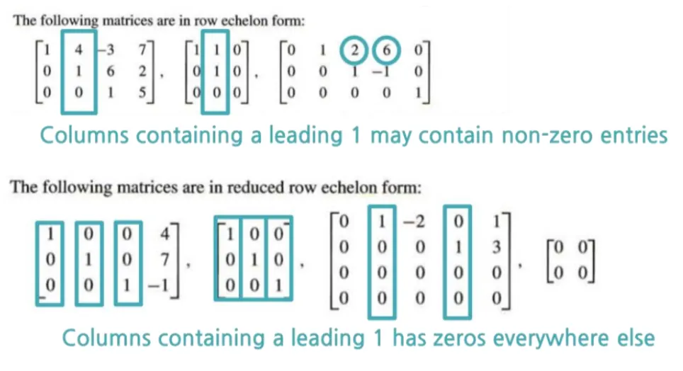
Reduced Row Echelon Form (RREF)
Reducing the augmented matrix into a RREF allows us to directly “read off” the solution
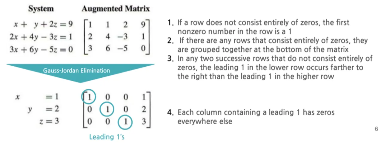
Gauss-Jordan Elimination
Gauss Elimination (Forward Phase): uses the three aforementioned elementary row operations to introduce zeros below the leading 1’s.
Jordan Elimination (Backward Phase): uses the three aforementioned elementary row operations to introduce zeros above the leading 1’s.
Applications of Linear Systems of Equations
GPS Systems
Produce four equations with four unknown variables, (x, y, z and t). The coordinates of a
satellite’s position at different times can be used to find the satellite’s position as a function of time.

Satellite | Satellite Position | Time |
1 | (1.12, 2.10, 1.40) | 1.06 |
2 | (0.00, 1.53, 2.30) | 0.56 |
3 | (1.40, 1.12, 2.10) | 1.16 |
4 | (2.30, 0.00, 1.53) | 0.75 |
Network Analysis
Using the conservation of flow (water, charge, vehicles), elaborate pipe/circuit/road systems can be designed and analyzed.


Balancing Chemical Equations
Set up a system of equations where the coefficients of elements in a chemical reaction
are represented as unknown variables.

Geometric Transformations Using Matrices (AI-friendly)
Transformation Matrices
Operator
Rotation about the positive x-axis through an angle θ
Rotation about the positive y-axis through an angle θ
Rotation about the positive z-axis through an angle θ
Illustration


Standard Matrix
Proof/ Derivation of Transformation Matrices
1.
Rotation about origin

2.
Reflection across line that makes an angle with the -axis

3.
Orthogonal Projection onto a line

Composite Transformations
Rotation about the origin through an angle
Reflection about the line through the origin making an angle with the positive -axis
Orthogonal projection onto the line through the origin making an angle with the positive -axis

The following theorem shows that the composition of two linear transformations is itself a linear transformation.
If and are both linear transformations, then is also a linear transformation,
Example 1: Composing Rotations in
Let be the rotation about the origion of through the angle , and let be the rotation about the origin through the angle . The standard matrices for these rotations are
and (4)
The composition
first rotates through the angle and then rotates through the angle , so the standard matrix for should be
(5)
To confirm that this is so let us apply Formula (2). According to that formula the standard matrix is
=
which agrees with (5).
Example 2: Composing Reflections
By Formula (18) of Section 6.1, the matrices
and
represent reflections about lines through the origin of making angles of and with the -axis, respectively. Accordingly, if we first reflect about the line making the angle and then about the line making the angle , then we obtain a linear operator whose standard matrix is
Comparing this matrix to the matrix in formula (16) of Section 6.1, we see that this matrix represents a rotation about the origin through an angle of . Thus, we have shown that
This results is illustrated in Figure 6.4.2.
