Curve Fitting & Regression Techniques

Sample Research Questions

•

How can regression techniques be used to explain the relationship between xxx and yyy?

•

Predicting the yyy value based on multiple input factors x1x_1x1​, x2x_2x2​, x3x_3x3​?

•

How can interpolation methods can be used to generate the simplest possible curve passing through nnn data points?

How can [Regression Technique] be used to explain the relationship between [explanatory variable #1, #2, #3...] and [dependent variable]

Linear Regression

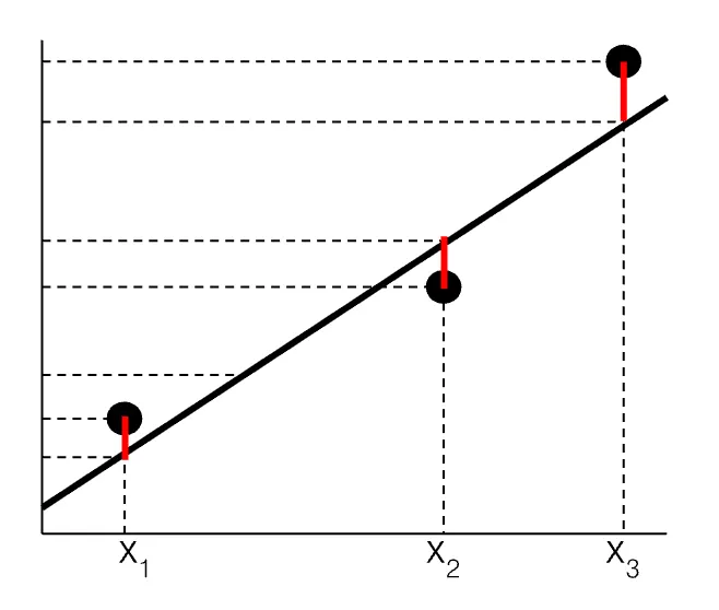
Suppose we have

n

non-collinear data points,

(x_1, y_1)

(x_2, y_2)

,…,

(x_n, y_n)

A linear regression model,

\hat y=ax+b

, may be defined to predict a value of

y

for each corresponding input value of

x

Depending on how the line is drawn, some predicted values

\hat {y_i}

are less than the actual value

y_i

\hat {y_1}=ax_1+b

and

\hat y_3=ax_3+b

underestimate the value of

y_1

and

y_3

respectively.

In other cases, the predicted value of

\hat {y_i}

is greater than the actual value of

y_i

\hat {y_2}=ax_2+b

, for example, overestimates the value of

y_2

Given that an infinite combination of coefficients

(a, b)

are possible, which linear equation

\hat y=ax+b

would be the curve of best fit offering the most accurate representation of all individual data points?

Key Questions

•

Is there a metric that quantifies and compares how closely linear regression models fit over a set of data points?

•

Should the regression model prioritize fitting certain data points more closely than others or should it aim to minimize the overall error across all data points?

Sum of Squared Errors (SSE) is a collective measure of error that penalizes both positive and negative deviations from all data points equally.

Linear Regression seeks to find the set of coefficients that minimizes SSE

Minimize

\sum _{i=1}^n(y_i-\hat{y_i})^2

Investigation:

Find

(a,b)

such that:

(y_1-ax_1-b)^2+ (y_2-ax_2-b)^2+(y_3-ax_3-b)^2

is minimized.

The optimal solution,

(a^*,b^*)

, provides coefficients for line of best fit that minimizes SSE.

\hat y=a^*x+b^*

Extension:

•

What other loss functions, other than SSE, can be used to penalize deviations of the model from data points to guide the optimal selection of model parameters (a,b)(a, b)(a,b)?

•

What if more complex, non-linear regression models like y^=ax2+bx+c\hat y=ax^2+bx+cy^​=ax2+bx+c promise a better fit?

Polynomial Interpolation

Extending the previous discussion of linear regression models in the form,

\hat y=ax+b

the polynomial interpolation method finds a polynomial function that fits a set of data points exactly.

Polynomial Interpolation Theorem

Given any

n+1

points,

(x_0, y_0)

(x_1, y_1)

,…,

(x_n, y_n)

, in the

xy

-plane with distinct

x

-coordinates such that

x_0<x_1<x_2…<x_n

, there is a unique

n

th degree polynomial passing through each of these points.

y= a_nx^n+a_{n-1}x^{n-1}+…+a_2x^2+a_1x+a_0

Substituting known pairs of

x

’s and

y

’s that the polynomial function passes through, the following system of equations must be satisfied:

y_0=a_nx_0^n+a_{n-1}x_0^{n-1}+…+a_2x_0^2+a_1x_0+a_0

y_1=a_nx_1^n+a_{n-1}x_1^{n-1} +…+a_2x_1^2+a_1x_1+a_0

…

y_n=a_nx_n^n+a_{n-1}x_n^{n-1}+…+a_2x_n^2+a_1x_n+a_0

Investigation

Find a cubic polynomial function whose graph passes through these four points:

(1,2)

(2,-3)

(3,-5)

(4,0)

Solve system of equations to find coefficients:

p(x)=a_3x^3+a_2x^2+a_1x+a_0

p(1)=2, ~p(2)= -3,~ p(3)=-5, ~p(4)=0

2=a_31^3+a_21^2+a_11+a_0

-3=a_32^3+a_22^2+a_12+a_0

-5=a_33^3+a_23^2+a_13+a_0

0=a_34^3+a_24^2+a_14+a_0

Extension:

•

Systematic approaches to reliably obtain solutions to large systems of equations with mmm equations and nnn unknown variables (in the HL syllabus, we typically worked with m≤3m≤3m≤3, n≤3n≤3n≤3)

•

Lagrange polynomial interpolation

y = \frac{(x - x_1)(x - x_2)\cdots(x - x_n)}{(x_0 - x_1)(x_0 - x_2)\cdots(x_0 - x_n)} y_0 + \frac{(x - x_0)(x - x_2)\cdots(x - x_n)}{(x_1 - x_0)(x_1 - x_2)\cdots(x_1 - x_n)} y_1 + \cdots + \frac{(x - x_0)(x - x_1)\cdots(x - x_{n-1})}{(x_n - x_0)(x_n - x_1)\cdots(x_n - x_{n-1})} y_n

Equivalently, we can use product notion:

y = \sum_{i=0}^{n} \left( y_i \prod_{\substack{j=0 \\ j \ne i}}^{n} \frac{x - x_j}{x_i - x_j} \right)

•

Newton polynomial interpolation

\begin{aligned}y &= b_0 + b_1(x - x_0) + b_2(x - x_0)(x - x_1) + \cdots + b_n(x - x_0)(x - x_1) \cdots (x - x_{n-1}) \\\\b_0 &= y_0 \\b_1 &= [y_0, y_1] = \frac{y_1 - y_0}{x_1 - x_0} \\b_2 &= [y_0, y_1, y_2] = \frac{ \frac{y_2 - y_1}{x_2 - x_1} - \frac{y_1 - y_0}{x_1 - x_0} }{x_2 - x_0} \\&\vdots \\b_n &= [y_0, y_1, \dots, y_n] = \frac{[y_1, y_2, \dots, y_n] - [y_0, y_1, \dots, y_{n-1}]}{x_n - x_0}\end{aligned}

•

Could we perform regression (curve fitting) for more than one independent variables?

Multiple Linear Regression

For a bivariate data set, regression equations modelled

y

as a single variate function of

x

$X$	$Y$
$x_1$	$y_1$
$x_2$	$y_2$
$x_3$	$y_3$

y= \beta_0+\beta_1x ,~ y=\beta_ 0+\beta_1x+\beta_2x^2

For multivariate data sets, a multitude of input variables are mapped to one composite output.

$X_1$	X2	$X_3$	$Y$
$x_{1,1}$	$x_{2,1}$	$x_{3,1}$	$y_1$
$x_{1,2}$	$x_{2,2}$	$x_{3,2}$	$y_2$
$x_{1,3}$	$x_{2,3}$	$x_{3,3}$	$y_3$

\hat y= \beta_0+\beta_1x_1+\beta_2x_2+\beta_3x_3 ,~ \hat y= \beta_0+\beta_1x_1+\beta_2x_2+\beta_3x_3+\beta_4x_1^2+\beta_5x_2x_3

Loss Function (SSE)

Similarly to classic linear regression, define a sum of squared error (SSE) metric loss function that penalizes deviations between the actual value of

y

and the predicted value of

y

Apply partial differentiation to solve for the optimal selection of coefficients that minimize the loss function,

L(\beta_0,\beta_1,\beta_2,\beta_3)

For

\hat y=\beta_ 0+\beta_1x_1+\beta_2x_2+\beta_3x_3

L(\beta_0,\beta_1,\beta_2,\beta_3)=\sum_{i=1}^n(y_i-\hat{y_i})^2

L(\beta_0,\beta_1,\beta_2,\beta_3)=\sum_{i=1}^n(y_i-\beta_0-\beta_1x_1-\beta_2x_2-\beta_3x_3)^2

Partial Differentiation

\frac{∂f(x,y,z)}{∂x}=\frac{f(x+h,y,z)-f(x,y,z)}h

Similar to the

\frac{df(x)}{dx}=0

condition, setting the partial differentiation to zero is a technique used for optimization, but for multivariate functions.

Investigation

\frac{∂L(\beta_0,\beta_1,\beta_2,\beta_3)}{∂\beta_0}=\frac{∂L(\beta_0,\beta_1,\beta_2,\beta_3)}{∂\beta_1}=\frac{∂L(\beta_0,\beta_1,\beta_2,\beta_3)}{∂\beta_2}=\frac{∂L(\beta_0,\beta_1,\beta_2,\beta_3)}{∂\beta_3}=0

Minimizing loss function

L

with respect to

\beta_0,\beta_1,\beta_2,\beta_3

gives rise to the least squares normal equations.

\left. \frac{\partial L}{\partial \beta_0} \right|_{\hat{\beta}_0, \hat{\beta}_1, \dots, \hat{\beta}_k} = -2 \sum_{i=1}^{n} \left( y_i - \hat{\beta}_0 - \sum_{j=1}^{k} \hat{\beta}_j x_{ij} \right) = 0\\\\ \left. \frac{\partial L}{\partial \beta_j} \right|_{\hat{\beta}_0, \hat{\beta}_1, \dots, \hat{\beta}_k} = -2 \sum_{i=1}^{n} \left( y_i - \hat{\beta}_0 - \sum_{j=1}^{k} \hat{\beta}_j x_{ij} \right) x_{ij} = 0 \quad \text{} j = 1, 2, \dots, k\\\\ n \hat{\beta}_0 + \hat{\beta}_1 \sum_{i=1}^{n} x_{i1} + \hat{\beta}_2 \sum_{i=1}^{n} x_{i2} + \cdots + \hat{\beta}_k \sum_{i=1}^{n} x_{ik} = \sum_{i=1}^{n} y_i\\\\ \hat{\beta}_0 \sum_{i=1}^{n} x_{i1} + \hat{\beta}_1 \sum_{i=1}^{n} x_{i1}^2 + \hat{\beta}_2 \sum_{i=1}^{n} x_{i1} x_{i2} + \cdots + \hat{\beta}_k \sum_{i=1}^{n} x_{i1} x_{ik} = \sum_{i=1}^{n} x_{i1} y_i\\\\ \hat{\beta}_0 \sum_{i=1}^{n} x_{ik} + \hat{\beta}_1 \sum_{i=1}^{n} x_{ik} x_{i1} + \hat{\beta}_2 \sum_{i=1}^{n} x_{ik} x_{i2} + \cdots + \hat{\beta}_k \sum_{i=1}^{n} x_{ik}^2 = \sum_{i=1}^{n} x_{ik} y_i

Extension

•

What are some real life situations or problems that invite the appropriate use of multiple linear regression?

•

How can we incorporate non-linear terms into multiple linear regression models?