

Price elasticity of Demand (PED)
•
given a change in P, does Qd change a lot or little? The concept of PED addresses this question.
•
PED: the measure of the responsiveness of Qd to changes in P.
◦
PED is calculated along a given D curve. In general, if Qd is highly responsive to price changes, D is referred to as being price elastic; if Qd is not very responsive, D is price inelastic.
The formula for PED
•
Because of the law of demand( inverse relationship between P and Q) PED has a negative value. However, PED is treated as if it were positive (absolute value).
•
Calculating PED for hamburgers:
Suppose the price of hamburgers increases from $5 per hamburger to $10 per hamburger and the quantity demanded falls from 200 hamburgers to 150 hamburgers. What is the PED for hamburgers?
Degrees of PED—theoretical range of values for PED
•
Price elastic demand (PED>1)
◦
% change in Qd > % change in P = the change in Q is proportionately larger than the change in P
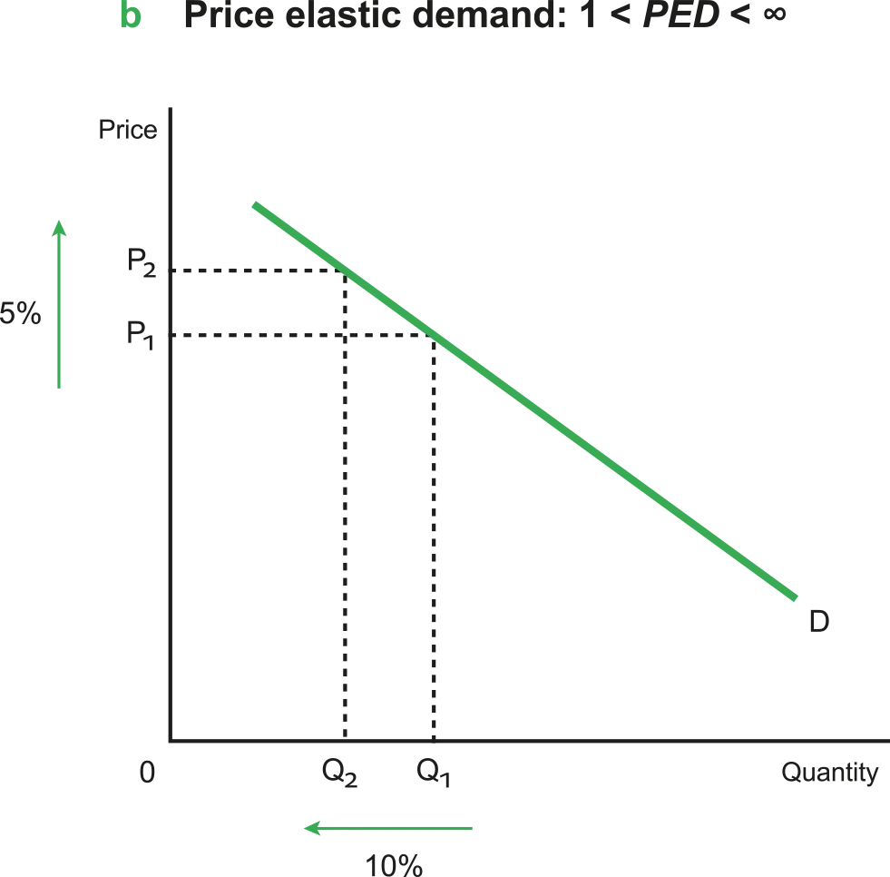
Figure 2.5.1 1 < PED < ∞
•
Price inelastic demand (0<PED<1)
◦
% change in Qd < % change in P and the change in Q is proportionately smaller than the change in P
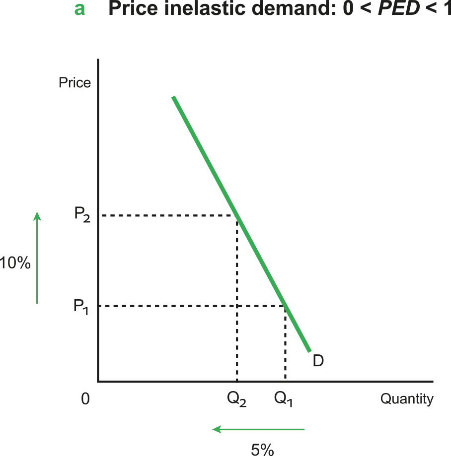
Figure 2.5.2 0 < PED < 1
In addition, there are 3 special cases when PED is constant (unchanging) along the full length:
•
Perfectly elastic demand (PED = ∞)

Figure 2.5.3 PED = ∞
◦
The % change in Qd resulting from a change in P is infinitely large.
◦
Special case used in economic theory to illustrate demand in perfect competition.
◦
When D is perfectly elastic, the D curve is horizontal.
•
Perfectly inelastic demand (PED=0)
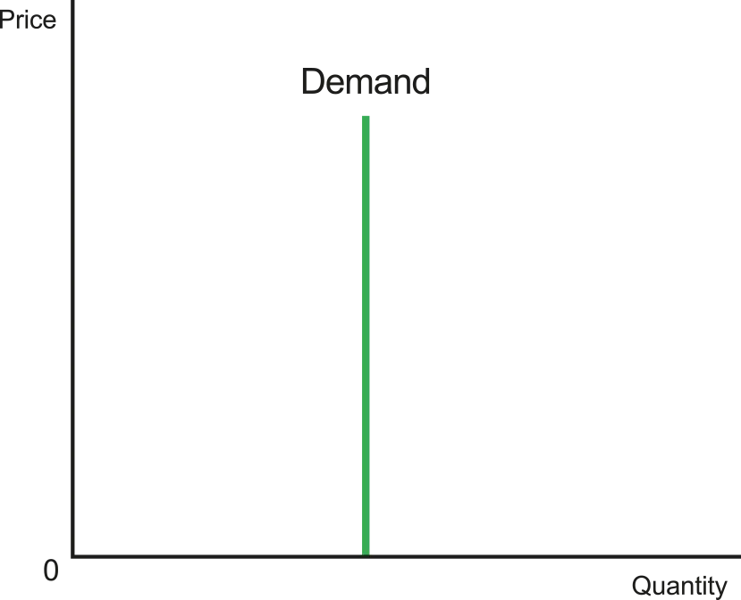
Figure 2.5.4 PED = 0
◦
The % change in Qd is zero; no matter how high P rises, Q demanded does not respond.
◦
This situation might be approached in cases of drug addiction.
◦
When D is perfectly inelastic, the D curve is vertical.
•
Unit elastic demand (PED=1)
◦
The % change in Qd = the % change in P = change in Q is proportionately equal to the change in P
◦
Theoretical idea that is unlikely to be found in the real world.
◦
When D is unit elastic, the D curve is a rectangular hyperbola.
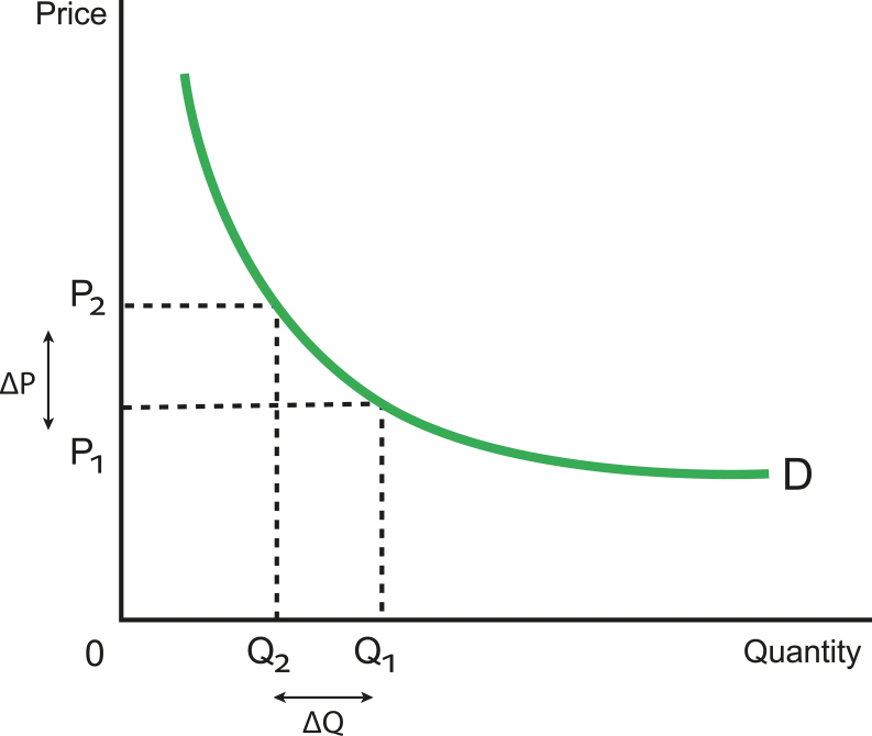
Figure 2.5.5 PED = 1
PED and the steepness of the D curve
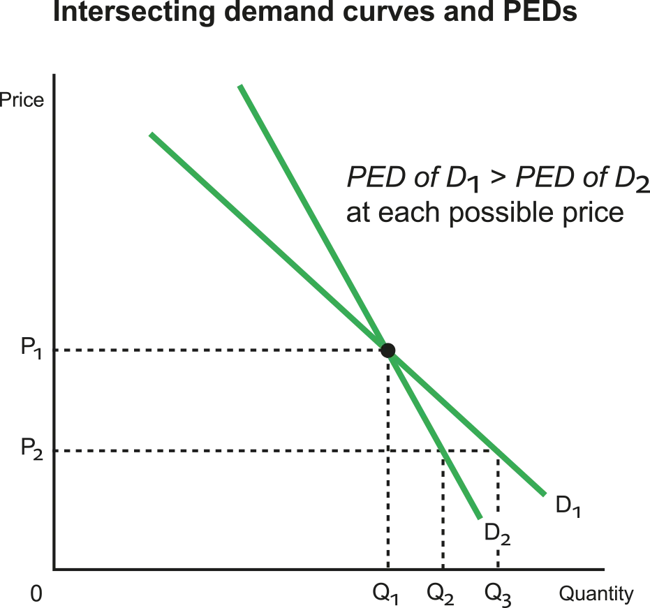
Figure 2.5.6 Demand curves and PEDs
•
In a diagram with two intersecting D curves, the flatter curve has the more elastic D for the same change in P.
•
D1 is flatter and more elastic than D2. If P falls from P1 to P2, the resulting % change in Q will be larger for D1 (an increase from Q1 to Q3) than for D2 (an increase from Q1 to Q2).
Changing PED along a straight line downward sloping D curve (HL only)
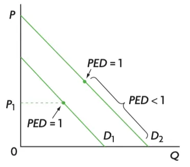
Figure 2.5.7 PED changes on the D curve
•
PED changes along the length of the curve, continuously falling as P decreases and Q increases.
•
D is price-elastic at high P and low Q, and price-inelastic at low P and large Q. At the midpoint of the D curve, there is a unit elastic D.
•
Therefore, the terms ‘elastic’ and ‘inelastic’ should not be used to refer to an entire D curve (except in the three cases where PED is constant) but only to a portion of the D curve corresponding to a particular P or P range.
Determinants of PED
1.
Number and closeness of substitutes
•
The more close substitutes a good has, the more elastic its demand → Greater its PED.
•
e.g. if P of strawberries increases consumers can switch to other fruits (e.g. apples) → high responsiveness (drop) of Q of strawberries demanded.
•
e.g. if P of gasoline increases, consumers have few alternatives → low responsiveness (drop) of Q of gasoline demanded.
•
Strawberries have price-elastic D; gasoline has price-inelastic D.
2.
Degree of necessity
•
Necessity = a good that is necessary to a consumer (contrasted with a luxury = a good that is not essential).
•
The more necessary a good, the less elastic its D → lower its PED.
•
e.g. Food is a necessity people cannot live without → if P of food increases, the Q of food demanded will drop insignificantly.
•
PED for necessities < PED for luxuries.
3.
Proportion of income spent on the good
•
The greater the proportion of income spent on a good, the more elastic its demand → greater its PED.
•
e.g. Comparing computers to pencils: since computers take up a larger proportion of consumer income than pencils, an increase in P of computers will be felt more strongly by consumers than an increase in P of pencils, leading to greater responsiveness (drop) in the Qd of computers.
•
PED for computers > PED for pencils.
4.
Time
•
The more time a consumer has available to make a decision to buy a good → more elastic D.
•
e.g. if P of gasoline increases, over a short time there will be a small drop in Qd, but over longer periods consumers can switch to other forms of transportation than cars → larger drop in Qd.
Importance of PED for firms and government decision-making
Knowledge of PED is important to firms seeking to maximise their revenue
•
Price-inelastic products = ↑ prices = boost revenue
•
Price-elastic products = ↓ prices = boost revenue
Knowledge of PED is important to Governments with regard to taxation and subsidies
•
Taxing price-inelastic products can increase tax revenue without significantly harming firms
◦
consumers are less responsive to price changes.
•
Subsidising price-elastic products can lead to a greater increase in quantity demanded
◦
Encourages consumption of merit goods such as electric vehicles
Relationship between PED and Total Revenue
Total Revenue (TR) = P x Q = a firm’s total earnings from selling its output. As P changes, TR may increase, decrease, or stay unchanged, depending on PED.
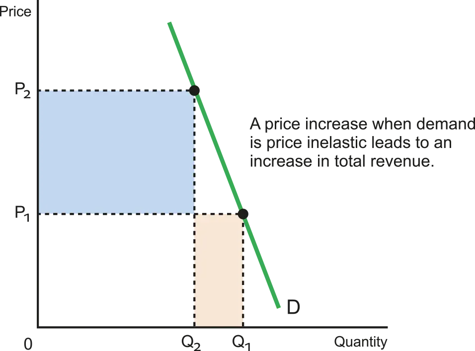
Figure 2.5.8 PED and total revenue
Elastic D (PED>1) → % change in Q > % change in P → P and TR change in opposite directions.
•
If P increases, TR falls.
◦
if P increases, Q falls proportionately more since the % decrease in Q is larger than the % increase in P → TR falls.
•
If P decreases, TR increases.
◦
if P falls, Q increases proportionately more since the % increase in Q is larger than the % decrease in P →TR increases.
Inelastic D (PED<1) → % change in Q < % change in P → P and TR change in the same direction.
•
If P increases, TR increases.
◦
if P increases, Q falls proportionately less since the % increase in Q is larger than the % decrease in Q →TR increases.
•
If P falls, TR falls.
◦
If P falls, Q increases proportionately less since the % decrease in P is larger than the % increase in Q → TR falls.
If D is unit elastic (PED=1).
•
A change in P does not cause any change in TR.
Firms must take PED into account when considering changes in the P of their product.
•
To increase TR, firms should:
◦
Elastic D: decrease P
◦
Inelastic D: increase P
•
Unit elastic D: If D is unit elastic, the firm is unable to change its TR by changing its P.
PED and indirect taxes
The more inelastic demand (lower the PED) for the taxed goods, the greater the government tax revenues.
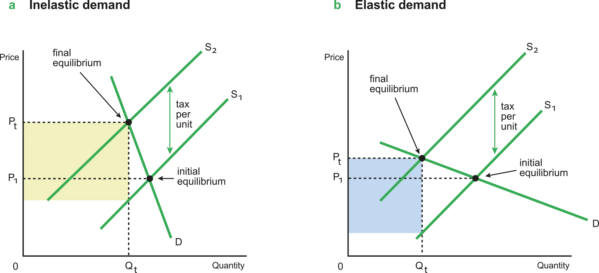
Figure 2.5.9 PED, indirect taxes and government tax revenue
•
The lower the PED for the taxed good(the more inelastic the D), the greater the government tax revenues.
•
When D is inelastic, an increase in P (due to tax) leads to a proportionately smaller decrease in QD → increase in TR
Reasons why the PED for primary commodities is generally lower than the PED for manufactured products (HL only)
•
Primary commodities: goods arising directly from the use of natural resources, or the factor of production ‘land’
◦
e.g., agricultural products, fishing and forestry products, extractive products ( oil, coal, minerals).
◦
Necessity, no substitutes & take up small proportions of income → Low PED
•
Manufactured products: goods produced by labour usually working together with capital as well as raw materials
◦
e.g. cars, computers, televisions).
◦
Luxuries, have substitutes & take up large proportions of income → High PED
◦
Exceptions: medications have low PED as they are necessitives & have no substitutes
Income elasticity of demand (YED)
•
Changes in income lead to changes in D. How, and how much does D change? The concept of YED addresses these questions.
•
YED: the measure of the responsiveness of D to changes in income, and involves D curve shifts.
The formula for YED
•
Calculating YED for clothes:
Suppose your income increases from $800 per month to $1000 per month, and your purchases of clothes increase from $100 to $140 per month. What is your YED for clothes?
Income elastic demand (service and luxury goods) and income inelastic demand (necessities)
•
YED>0: normal goods
◦
D for goods & income change in the same direction. (both increase or both decrease).
◦
Most goods are normal goods.
◦
e.g., food clothes
•
YED<0: inferior goods
◦
D for goods & income move in opposite directions (as one increases the other decreases).
◦
e.g., second hand clothes, used cars
•
YED<1: Necessities.
◦
Income inelastic DA % increase in income results in a smaller % increase in Qd.
◦
e.g. food, housing, clothing
•
YED>1: Luxuries
◦
= Income elastic D
◦
A % increase in income produces a larger % increase in Qd.
◦
e.g. jewellery, designer clothes, private education
•
What is a necessity and what is a luxury depends on income levels. For people with low incomes, even food and clothing can be luxuries. As income increases, certain items that used to be luxuries become necessities.
•
e.g. items like Coca-Cola and coffee for many poor people in less developed countries are luxuries, whereas for consumers in developed countries, they have become necessities.

Figure 2.5.10 Demand curve shifts in response to increases in income for different YEDs
•
In the case of necessities(YED<1), an increase in income will produce a relatively small rightward shift in the D curve; in the case of luxuries and services(YED>1), the rightward shift will be larger.
The Engel Curve
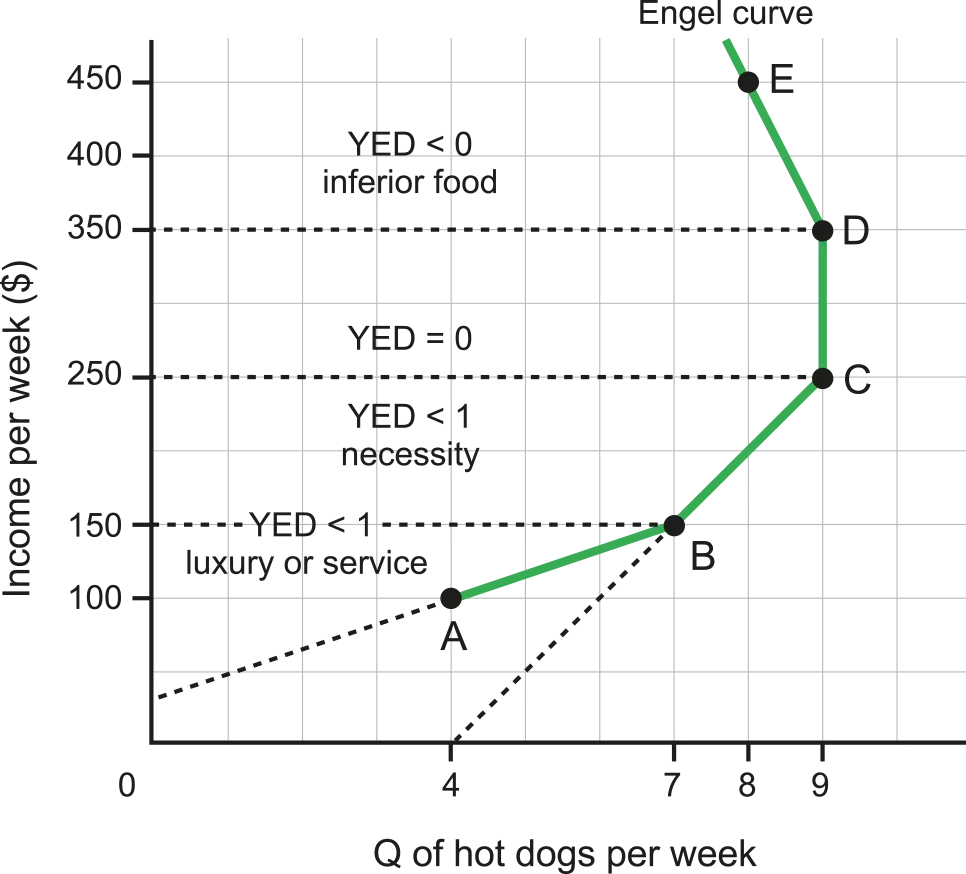
Figure 2.5.11 The Engel curve showing different YEDs
•
Engel curve diagram illustrates the following:
◦
YED>0 in the upward sloping part of the curve: Q and income both increase = indicates the good is normal.
◦
YED<0 in the downward sloping part of the curve: Q decreases as income increases = indicates the good is inferior.
◦
YED>1 in the upward sloping part of the curve: huge income ↑ = small QD ↑ = indicates the good is luxury. (3% ↑ in income = to a 10% ↑ in QD)
◦
0 → 1 in the upward sloping part of the curve: small income ↑ = huge QD ↑ = indicates the good is a necessity. (10% ↑ in income = to a 3% ↑ in QD)
•
The Engel curve can also show a continuum: at very low incomes, a good may be a luxury; as income increases, it becomes a necessity, and finally at high income levels, it becomes inferior.
◦
In the diagram, for very low levels of income under $150 per week, hot dogs are luxuries as YED>1. However, at higher levels of income above $350 per week, hot dogs are considered inferior as YED<0.
Factors that influence YED
•
YED is affected by various economic factors that alter workers' wages.
•
In recessions, wages typically decline, leading to increased demand for inferior goods and reduced demand for luxury goods.
•
Conversely, in economic upturns with rising wages, demand for luxury goods rises, while demand for inferior goods declines.
•
Other factors impacting income include minimum wage laws, taxation policies, and changes in international trade.
Importance of YED (HL only)
YED and for firms: the rate of expansion of industries
•
Producers may be interested in knowing YED of their product as this affects how rapidly D for it will grow as income changes.
•
In a growing economy with increasing incomes, manufacturing and service industries or goods and services with high YEDs(normal goods) will experience the most rapid increases in D.
•
In an economy that is experiencing a recession and falling incomes, primary industry or goods and services with negative YEDs (inferior goods) may experience rapid growth.
In explaining changes in the sector structure of the economy
•
Every economy has three sectors: the primary sector, the manufacturing sector, and the services sector.
•
As primary goods have a low YED while manufacturing products usually have high YEDs, and services as a group have the highest of all, these differing YED values mean that with economic growth, the relative size of the three sectors usually changes over time.
◦
Countries usually begin with very large primary sectors, but with economic growth and growth in incomes, manufacturing and services become increasingly important, as the primary sector shrinks in relative importance.
◦
This changing structure is the result of relatively more rapid growth in manufacturing and even faster growth in services, while the primary sector experiences slowest growth of all.