

Gallery view
Search
•
Demand: Is the amount of a good/service that a consumer is willing and able to purchase at a given price in a given time period.
•
Market demand: the sum of all individual buyers’ demand for a good.
The Law of Demand – the relationship between price and quantity demanded
The law of demand states that there is an inverse relationship between price and quantity demanded (QD), ceteris paribus
•
When the price ↑ the QD ↓
•
When the price ↓ the QD ↑
•
This is because as the P of a good increases, consumers are less willing and able to pay for the good.
Demand curve
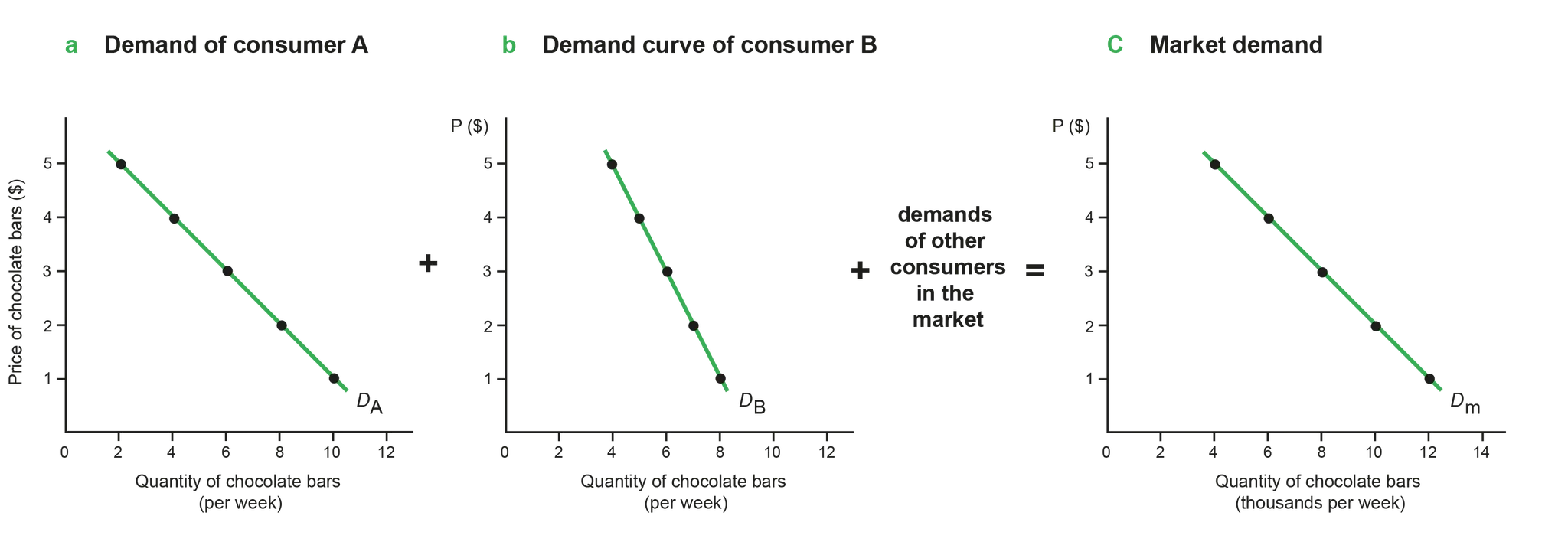
Figure 2.1.1 Market demand as the sum of individual demands
•
In a market of two buyers, market demand = individual D of buyer 1 + individual D of buyer 2.
•
The DS curve is downward sloping due to the law of demand (as P increases, Qds decreases).
Movement along a demand curve

Figure 2.1.2 Movement along and shifts of the demand curve
2.1. Demand
•
Supply: amount of a good/service that a producer is willing and able to supply at a given price in a given time period.
•
Market Supply: sum of all individual firms’ supplies for a good.
The Law of Supply – the relationship between price and quantity supplied
Law of Supply: states that there is a positive (direct) relationship between quantity supplied and price, ceteris paribus
•
When the price ↑ = the QS ↑
•
When the price ↓ = the QS ↓
The supply curve is sloping upward as there is a positive relationship between the price and quantity supplied
•
Rational profit maximising producers would want to supply more as prices increase in order to maximise their profits
Supply curve
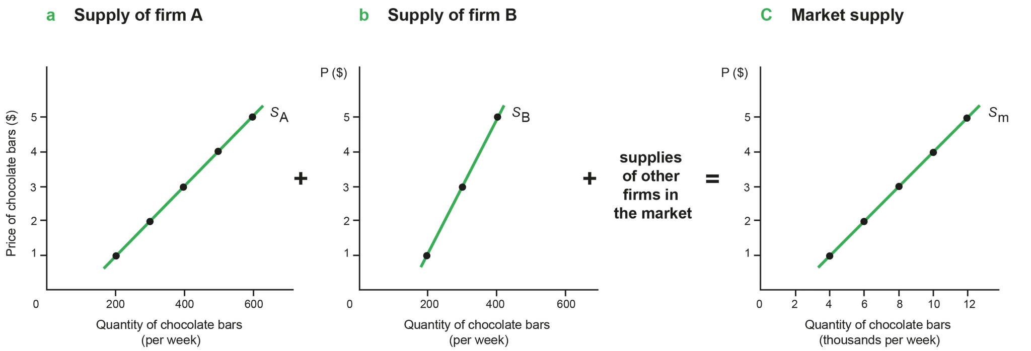
Figure 2.2.1 Market supply as the sum of individual supplies
•
In a market of two firms, market supply = S of firm 1 + S of firm 2.
•
The S curve is upward sloping due to the law of supply (as P increases, Qs increases).
2.2. Supply
Demand and supply curves forming a market equilibrium
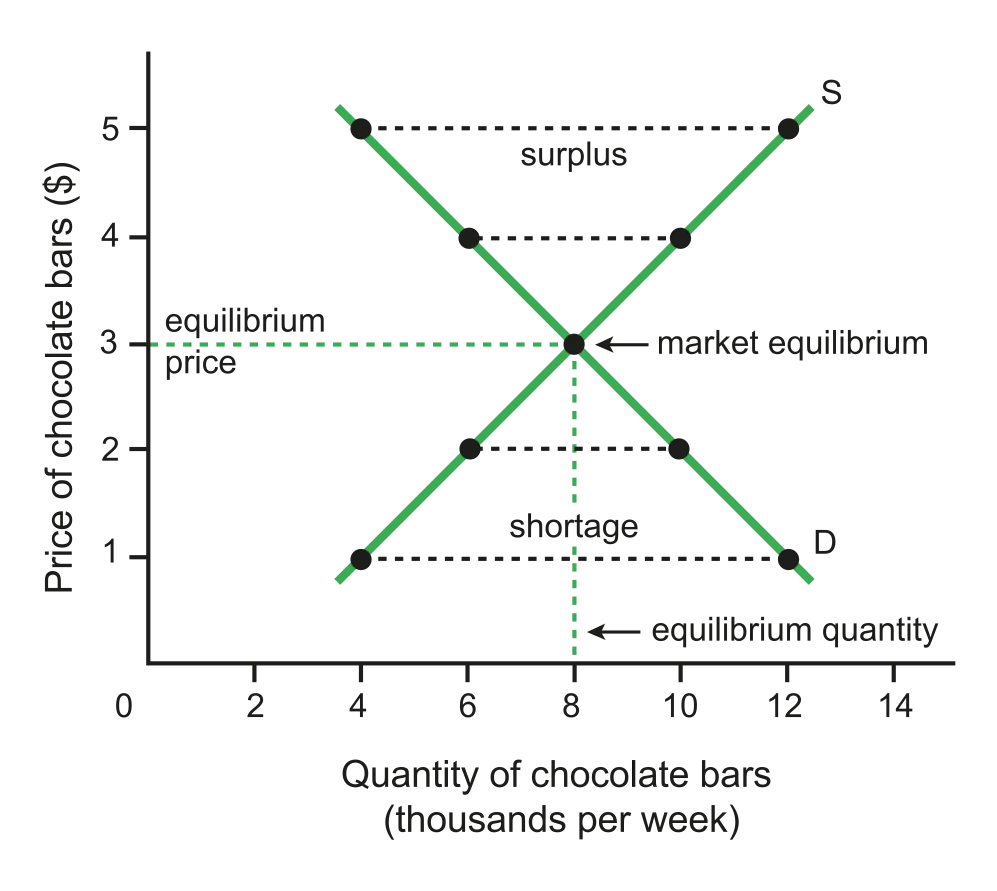
Figure 2.3.1 Market equilibrium
•
Market equilibrium: a position where the forces of D and S are in balance, and there is no tendency for P to change.
◦
In the diagram, market equilibrium is where D and S curves cross each other, determining equilibrium P ($3) and equilibrium Q (8000/week).
•
At every P other than equilibrium price ($3), Pe, there is market disequilibrium.
◦
If P>Pe → excess supply = surplus → Q demanded < Q supplied.
◦
If P<P3 → excess demand = shortage → Q supplied < Q demanded.
•
If there is a surplus, excess supply will ensure that P will decrease to Pe.
◦
Qd would increase while Qs would decrease, eliminating the surplus.
•
If there is a shortage, excess demand will ensure that P will increase to Pe.
◦
Qd would decrease while Qs would increase, eliminating the shortage.
Shifting the demand curve to produce a new market equilibrium
2.3. Competitive market equilibrium
Rational consumer choice
•
Free markets rely on the assumption of rational decision-making, where economic agents can assess the outcomes of their choices and recognize their net benefits.
•
Rational agents select choices that offer the highest utility or satisfaction, as per rational choice theory.
•
Economic theories presume individuals, firms, and governments aim to maximise satisfaction.
1.
Consumer Rationality: Individuals make choices based on rational calculations and available information.
2.
Utility Maximisation: Economic agents choose options that maximise their utility or satisfaction.
3.
Perfect Information: Rational choice theory assumes individuals have easy access to all information regarding goods and services to make optimal decisions.
Limitations of the Assumptions of Rational Consumer Choice
1.
Biases: impact the rational decision-making process by influencing our perceptions, judgments, and choices.
•
Rule of Thumb: Individuals often default to familiar choices based on past experiences, potentially overlooking better alternatives.
•
Anchoring and Framing: Anchoring bias involves relying heavily on initial information, while framing refers to how information presentation influences decisions.
•
Availability Bias: : People tend to overestimate the likelihood of events based on how easily they come to mind, influenced by personal experiences, media exposure, and emotional impact.
2.
Bounded Rationality Theory: People often make decisions without all necessary information due to time constraints and technical complexities.
•
Overwhelming choices, like in supermarkets, can lead to irrational decisions.
2.4. Critique of maximising behaviour of consumers and producers (HL only)
Price elasticity of Demand (PED)
•
given a change in P, does Qd change a lot or little? The concept of PED addresses this question.
•
PED: the measure of the responsiveness of Qd to changes in P.
◦
PED is calculated along a given D curve. In general, if Qd is highly responsive to price changes, D is referred to as being price elastic; if Qd is not very responsive, D is price inelastic.
The formula for PED
Price Elasticity of Demand (PED) =%Δ in P%Δ in Qd
•
Because of the law of demand( inverse relationship between P and Q) PED has a negative value. However, PED is treated as if it were positive (absolute value).
•
Calculating PED for hamburgers:
Suppose the price of hamburgers increases from $5 per hamburger to $10 per hamburger and the quantity demanded falls from 200 hamburgers to 150 hamburgers. What is the PED for hamburgers?
46−4200150−200=42200−50=400−200=−1/2=>1/2
Degrees of PED—theoretical range of values for PED
•
Price elastic demand (PED>1)
◦
% change in Qd > % change in P = the change in Q is proportionately larger than the change in P
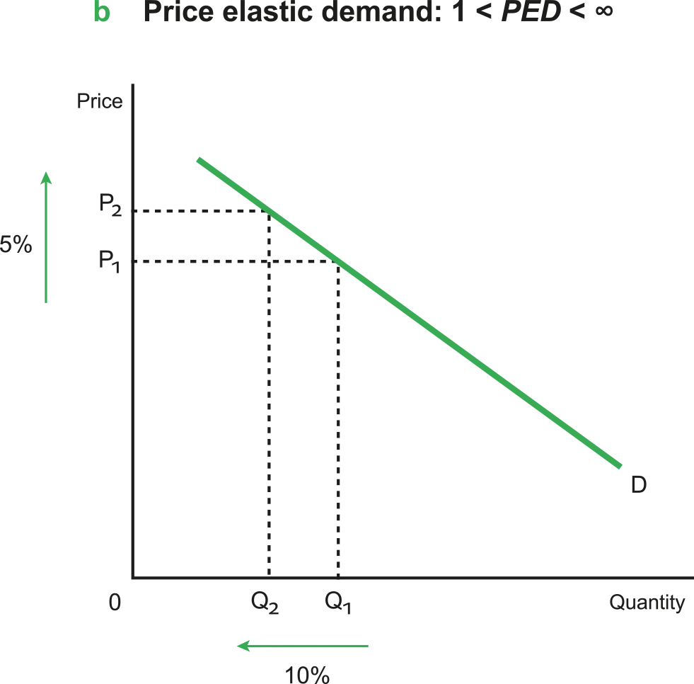
Figure 2.5.1 1 < PED < ∞
2.5. Elasticities of demand
Price elasticity of supply (PES)
•
According to the law of supply, an increase in P also results in an increase in Q supplied (Qs), and vice versa. Now, we ask, given a change in P, does Qs change a lot or little? The concept of PES addresses this question.
•
PES: the measure of the responsiveness of Qs of a good or service to changes in P, and PES is calculated along a given S curve.
The formula for PES
Price Elasticity of Supply (PES) =%Δ in P%Δ in Qs
•
Calculating PES for cabbages:
Suppose the price of cabbages increases from $2 per kg to $5 per kg and the quantity of cabbages supplied increases from 1000 hamburgers to 1100 tonnes per season. What is the PES for cabbages?
25−210001100−1000=231000100=1.50.1=0.666…=>0.67(2 d.p.)
Degrees of PES—theoretical range of values for PES
•
Price elastic supply (PES>1)
◦
% change in Qs > % change in P → Qs is relatively responsive to changes in P
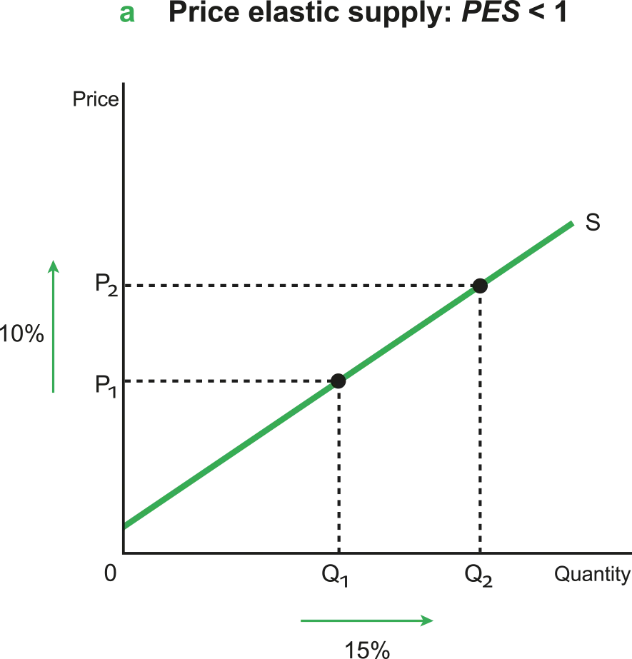
Figure 2.6.1 PES > 1
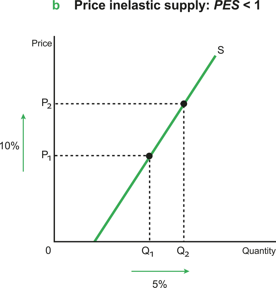
Figure 2.6.2 PES < 1
2.6. Elasticities of supply
Reasons for government intervention in markets
Influencing market outcomes in order to:
1.
Earn government revenue
•
Governments earn revenue through indirect taxes, which are taxes on goods and services.
•
The more price inelastic the demand for the good is, the greater the amount of tax revenue earned.
2.
Support firms
•
To support small firms that have just been set up and require financial assistance.
•
Support firms in an industry whose growth the government would like to encourage (e.g. environmental-friendly firms).
3.
Support households on low incomes
•
Subsidies, price ceilings, direct provision of services (e.g. free provision of education and health care).
•
Transfer payments, which include unemployment benefits, child benefits, maternity benefits, etc.
4.
Influence level of production
2.7. Role of government in microeconomics
Understanding Market Failure
•
In a free market, price mechanism determines efficient allocation of scarce resources
◦
Scarce resources include land, labour, capital, and entrepreneurship
•
Market failure occurs when:
◦
Allocation of resources is less than optimal
◦
Society's needs aren't effectively met by market mechanisms
Externalities occur when there is an external impact on a third party not involved in the economic transaction between the buyer and seller e.g. passive smoking is considered to be a negative externality
•
Can be either positive or negative, known as spillover effects
•
Affect either production or consumption side of the market
Public goods are beneficial to society but are underprovided by a free market (E.g. Vaccination)
•
Non-excludable and nonrivalrous in consumption
•
Little opportunity for sellers to make profits
Common pool resources are resources with no private ownership, they are collectively shared and are finite (used up) in consumption (E.g. Fishing grounds)
•
These resources are non-excludable and rivalrous (limited in supply)
Market failure is created where the allocation of resources is not efficient from society's perspective.
•
Overprovision of demerit goods = over-allocation of resources (e.g. cigarettes)
•
Underprovision of public goods and merit goods = under-allocation of resources (e.g. school)
•
Common pool resources = overuse of a finite resource
2.8. Market Failure – Externalities and common pool or common access resources
Characteristics of Public Goods
Private Goods:
•
Excludable and Rivalrous: Firms can provide private goods to generate profits because they can exclude customers through pricing mechanisms, and there's rivalry among consumers for limited supply.
•
Profit Generation: Exclusion and rivalry enable firms to generate profits.
Public Goods:
•
Non-Excludable and Non-Rivalrous: Public goods, like roads and national defence, are beneficial to society but not provided by private firms because they lack exclusability and rivalry.
•
Government Provision: Governments often provide public goods due to their non-excludable and non-rivalrous nature.
Free Rider Problem:
•
Non-Payment by Consumers: If firms attempt to provide public goods, consumers may realise they can access them without paying.
•
Free Riding: Consumers who can access the goods without payment may stop paying, leading to under-provision by firms over time.
Government Intervention in Response to Public Goods
1.
Do Nothing:
•
No provision is offered.
•
Public goods remain under-provided.
2.9. Market Failure: Public Goods
Understanding Asymmetric Information
Information Gaps and Market Failure
•
Perfect Information Assumption: Free markets assume perfect information, where buyers and sellers have equal knowledge about goods/services (symmetric information).
•
Asymmetric Information: In reality, buyers and sellers often have different levels of information (asymmetric information), leading to market distortions.
•
Market Distortions: Asymmetric information leads to distortions in market outcomes, resulting in over-provision or under-provision of goods/services.
•
Examples:
◦
Over-provision: Goods/services with undisclosed harmful effects (e.g., VW emissions scandal) are sold in higher quantities, leading to misallocation of resources.
◦
Under-provision: Goods/services with undisclosed benefits are sold in lower quantities, causing a shortage of these products and underutilization of resources.
Implications
•
Markets may not reach socially optimal prices and quantities due to information gaps.
•
Market interventions or regulations may be needed to address these distortions and improve allocative efficiency.
Adverse Selection
Arises when one party (typically the buyer) has better knowledge of their risk profile than the other party (seller).
•
Example: In insurance markets, individuals with higher risk (e.g., pre-existing conditions) are more motivated to buy insurance, leading to a higher proportion of higher-risk individuals in the risk pool.
•
Consequences: Imbalance in the risk pool may lead insurers to raise premiums, making insurance less affordable for lower-risk individuals and causing market failure.
•
Mitigation: Insurance companies may use strategies like risk-based pricing or medical underwriting to accurately reflect the risk profile of insured persons.
2.10. Market Failure: Asymmetric Information
Market Structures
Market structures refer to the characteristics of the market in which firms or industries operate. These include:
•
Number of Buyers: The quantity of consumers purchasing goods/services.
•
Number and Size of Firms: The quantity and scale of businesses operating in the market.
•
Type of Product: Whether products are homogenous (identical) or differentiated.
•
Barriers to Entry and Exit: Obstacles hindering or facilitating new firms entering or leaving the market.
•
Degree of Competition: The level of rivalry between firms.
Types of Market Structures
1.
Perfect Competition: A theoretical market structure with many buyers and sellers offering homogenous products, no barriers to entry/exit, and perfect information.
2.
Imperfect Competition: Market structures deviating from perfect competition, including:
•
Monopolistic Competition: Many firms with differentiated products (e.g., nail salons).
•
Oligopoly: A few large firms dominate, each with significant market power.
•
Monopoly: A single firm controls the entire market, influencing supply and prices.
Market Failure and Abuse of Market Power
Market failure can result from the abuse of market power, which is characterised by:
2.11. Market Failure: Market Power