

•
Supply: amount of a good/service that a producer is willing and able to supply at a given price in a given time period.
•
Market Supply: sum of all individual firms’ supplies for a good.
The Law of Supply – the relationship between price and quantity supplied
Law of Supply: states that there is a positive (direct) relationship between quantity supplied and price, ceteris paribus
•
When the price ↑ = the QS ↑
•
When the price ↓ = the QS ↓
The supply curve is sloping upward as there is a positive relationship between the price and quantity supplied
•
Rational profit maximising producers would want to supply more as prices increase in order to maximise their profits
Supply curve
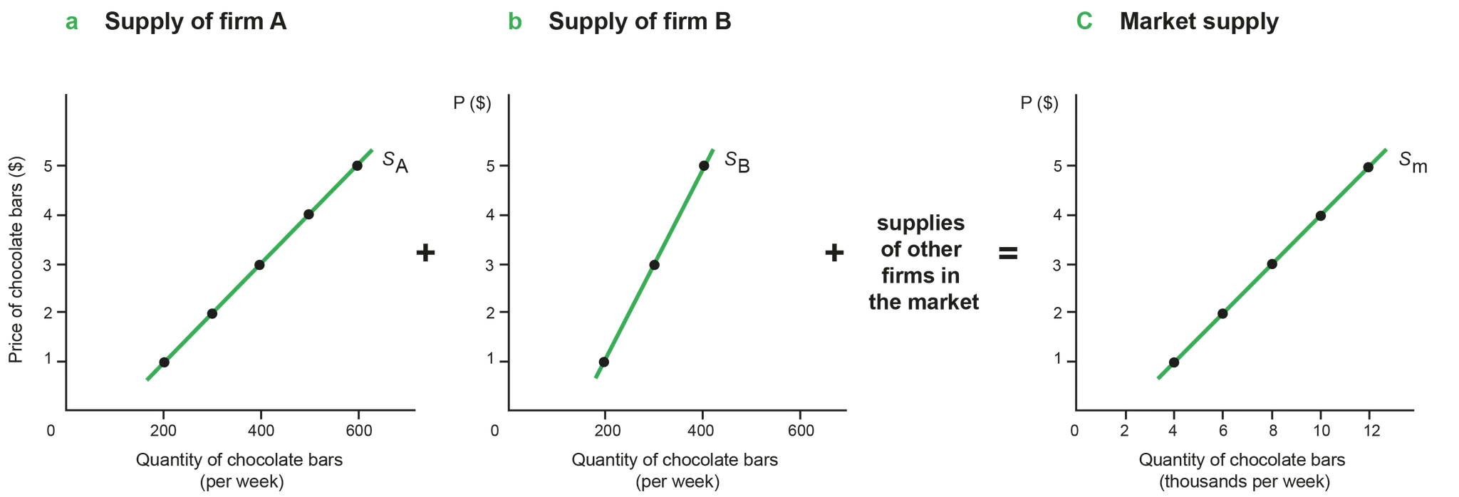
Figure 2.2.1 Market supply as the sum of individual supplies
•
In a market of two firms, market supply = S of firm 1 + S of firm 2.
•
The S curve is upward sloping due to the law of supply (as P increases, Qs increases).
Vertical Supply curve

Figure 2.2.2 The vertical supply curve
•
Vertical Supply: Qs is independent of P; even as P increases, Qs remains constant.
•
2 reasons for vertical supply:
1.
No time to produce more of it (e.g. fixed quantity of tickets in the theatre).
2.
No possibility of ever producing more of it (e.g. original paintings and sculptures of famous artists and original antiques).
Movement along a supply curve

Figure 2.2.3 Movements along the supply curve
•
Only caused by a change in P of the good.
•
According to the law of supply, if P increases, Q increases = upward movement from A to B.
•
The change in Q due to a change in P is called a change in quantity supplied.
Shift of the supply curve
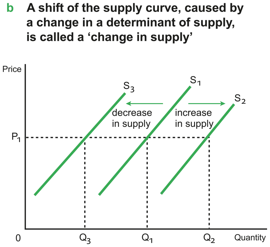
Figure 2.2.4 Shifting of the supply curve
•
Only caused by a change in non-price determinants of supply.
•
Rightward shift = increase in S, Leftward shift = decrease in S.
•
The change in Q due to the shifts in S is called a change in supply.
Non-price determinants of supply
1.
Costs of production
•
As prices of factors of production (e.g. wage for labour) increase, production becomes less profitable, thus S decreases.
2.
Technology
•
New improved technology lowers the cost of production, making production more profitable, thus S increases.
3.
Prices of related goods: competitive supply
•
Competitive supply: two or more products that compete for the use of the same resources (e.g. farmer can grow corn and wheat).
•
If P of corn increases, farmers switch to corn production as it is more profitable → S of wheat falls.
4.
Prices of related goods: joint supply
•
Joint supply: two or more products that are derived from the same product (e.g. butter and cheese both from whole milk).
•
Increase in P of butter means an increased S of butter an increase in S of cheese.
5.
Firm price expectation
•
If firms predict future P to rise, they may withhold some of their S now to sell it at a higher P in the future → fall in S in the present.
6.
Taxes (indirect taxes or taxes on profit)
•
Imposition of a new tax or increasing existing tax represents a higher cost of production, so S falls.
7.
Subsidies
•
Subsidy = payment made by the government to firms (encourage production).
•
Introduction of subsidy represents a fall in the cost of production, so S increases.
8.
The number of firms
•
Increase in the number of firms producing the good increases S, since market supply is the sum of all individual supplies.
9.
‘Shocks’, or sudden unpredictable events
•
e.g. weather conditions in the case of agricultural products and wars.
•
RWE: Louisiana Oil Spill in 2010 → S of locally produced seafood falls.
Assumptions underlying the Law of Supply (HL only)
1.
Law of diminishing marginal returns
•
Short run and Long run in Microeconomics.
◦
Short run: the time period during which at least one input is fixed and cannot be changed by the firm.
◦
Long run: the time period during which all inputs can be changed. There are no fixed inputs; all inputs are variable.
•
The meaning of marginal product.
◦
Total product: the total quantity of output produced by a firm (e.g. cabbage).
◦
Marginal product: additional unit of output produced by one additional unit of a variable input (e.g. labour).
Number of workers (the variable input) | Total product (kilos of cabbage) | Marginal product (kilos of cabbage) |
0 | 0 | - |
1 | 10 | 10 |
2 | 30 | 20 |
3 | 60 | 30 |
4 | 80 | 20 |
5 | 90 | 10 |
•
Law of diminishing marginal returns: As more of a variable factor of production (e.g. labour) is added to fixed factors (e.g. capital), there will initially be an increase in productivity
◦
However, a point will be reached where adding additional units of the factor (e.g. hiring an extra worker) begins to decrease productivity due to the relationship between labour and capital
•
Relationship between marginal product and marginal cost.
◦
When MP increases, MC decreases; when MP is at a maximum, MC is at a minimum.
▪
When the MP of an additional worker increases, the cost of an additional unit of output falls.
•
The firm’s supply curve is a portion of the upward sloping part of the MC curve.

Figure 2.2.5 Marginal product and cost curves