

Price elasticity of supply (PES)
•
According to the law of supply, an increase in P also results in an increase in Q supplied (Qs), and vice versa. Now, we ask, given a change in P, does Qs change a lot or little? The concept of PES addresses this question.
•
PES: the measure of the responsiveness of Qs of a good or service to changes in P, and PES is calculated along a given S curve.
The formula for PES
•
Calculating PES for cabbages:
Suppose the price of cabbages increases from $2 per kg to $5 per kg and the quantity of cabbages supplied increases from 1000 hamburgers to 1100 tonnes per season. What is the PES for cabbages?
Degrees of PES—theoretical range of values for PES
•
Price elastic supply (PES>1)
◦
% change in Qs > % change in P → Qs is relatively responsive to changes in P
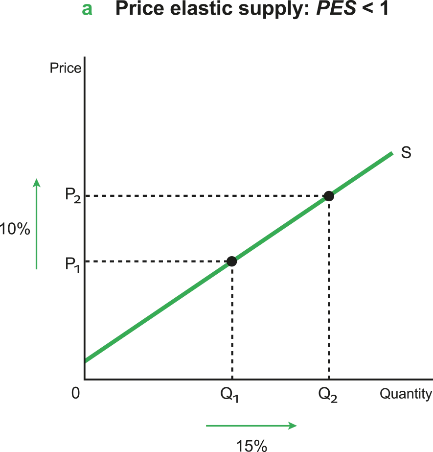
Figure 2.6.1 PES > 1
•
Price inelastic supply (PES<1)
•
% change in Qs < % change in P → Qs is relatively unresponsive to changes in P.
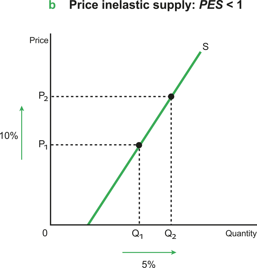
Figure 2.6.2 PES < 1
In addition, there are 3 special cases when PES is constant (unchanging) along the full length:
•
Perfectly elastic supply (PES = ∞)

Figure 2.6.3 PES = ∞
◦
% change in Qs = infinite → Qs is infinitely reponsive to P
◦
Horizontal S curve = A small change in P leads to an infinitely large change in Qs.
◦
Special case used in economic theory to illustrate world supply in international trade.
•
Perfectly inelastic supply (PES=0)
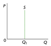
Figure 2.6.4 PES = 0
◦
% change in Qs = 0 → Qs is completely unresponsive to P
◦
Vertical S curve = a change in P leads to no change in Qs
◦
eg. original antique furniture and famous paintings have such a zero responsiveness.
•
Perfectly inelastic supply (PES=1)
Figure 2.6.5 PES = 1
◦
% change in Qs = % change in P → Qs in completely unresponsive to P
◦
S curve cuts the origin = % change in Q is proportionately equal to the change in P.
◦
Theoretical idea that is unlikely to be found in the real world.
Determinants of PES
1.
Length of time
•
The longer the time period a producer has to respond to P changes, the more elastic the S (higher PES)
•
Short time → Producer may be unable to respond to P changes
◦
e.g., unable to obtain all necessary resources and technology in order to increase output in response to a P increase
•
Long time → producer is able to respond to P changes
2.
Mobility of factors of production
•
The more quickly and easily necessary resources can be moved from one type to another where P is increasing, the more elastic the supply
3.
Unused capacity
•
The more unused capacity exists, the more elastic the supply.
•
Unused capacity (machine, quipment, labor) exists → easy for firms to respond with increased output to P increase by making use of the unused resources → high PES
4.
Ability to store stocks
•
The higher the ability to store stocks, the more elastic the S.
•
If a firm can store stocks easily and inexpensively, then in the event of a P increase firms can release available stock that can be sold in the market. → high PES
5.
Rate at which costs increase
•
The higher the rate at which costs increase, the more inelastic the S.
•
Costs of producing extra output increases rapidly → firms have difficulty expanding their output since they are unlikely to incur large costs → low PES
•
e.g. if P of fertiliser is rising rapidly, thus raising the farm’s cost of production, the farmer will find it more difficult to expand output quickly → low PES.
Reasons why the PES for primary commodity is generally lower than the PES for manufactured products (HL only)
•
Why low PES for primary commodities & high PES for manufactured products?
◦
Primary commodities need more time than manufactured products to be produced or extracted.
◦
e.g., agricultural products need to go through their natural growing time to respond to P changes.
A Comparison of the PES of Primary Commodities & Manufactured Products
PES Factor | Primary Commodities - Inelastic (PES = 0-1) | Manufactured Goods - Elastic (PES = >1) |
Mobility of the factors of production | When the price of a particular agricultural commodity rises, farmers cannot swiftly switch to producing a different crop. | Greater flexibility to switch production to alternative goods in response to price changes results in a higher PES. |
The rate at which costs of production (MC) increase | Production of primary commodities faces inherent constraints like longer production cycles. Cost to produce one more unit of output is relatively high. | The additional costs of supplying mass-produced manufactured products are generally lower due to the ease of adding extra units to production output. |
The ability to store goods | Perishable agricultural have limited storage capabilities short-term supply responsiveness | Can be stored longer without deterioration/spoilage
Allows firms to respond to price changes by adjusting the quantity supplied from existing stock |
Spare production capacity | Output is relatively labour or land-intensive, imposing limits on spare production capacity | Output is often generated using machinery, allowing for more capacity when producing manufactured products |
Time period | To grow or extract primary commodities is much longer | Short time period |