

Aggregate demand
Aggregate demand(AD): total spending on domestic goods and services at average price levels per period of time.
•
AD = C + I + G + (X-M)
◦
C = consumption expenditures
◦
I = investment expenditures
◦
G = government expenditures
◦
X-M = net export (export - import)
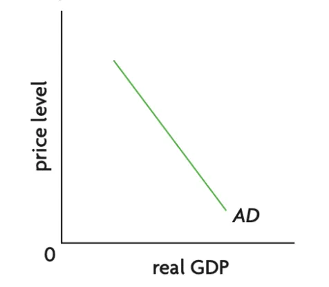
Figure 3.2.1 The aggregate demand curve
Why is the AD curve downward sloping?
Wealth effect | Trade effect | Interest rate effect |
average price level(APL) ↑ → real value of money people possess ↓ (i.e. people feel ‘poorer’) → consumer expenditure (C) ↓ → C is a component of AD → upward movement along AD | APL ↑ → exports become less competitive abroad // imports seem more attractive at home country → value of net export (X-M) ↓ → X-M is component of AD → upward movement along AD . | APL ↑ → demand for holding money ↑ → C and investment expenditure (I) ↓
(i.e. people and firms will borrow less from banks to buy durables and capital equipment) → C & I are components of AD → upward movement along AD . |
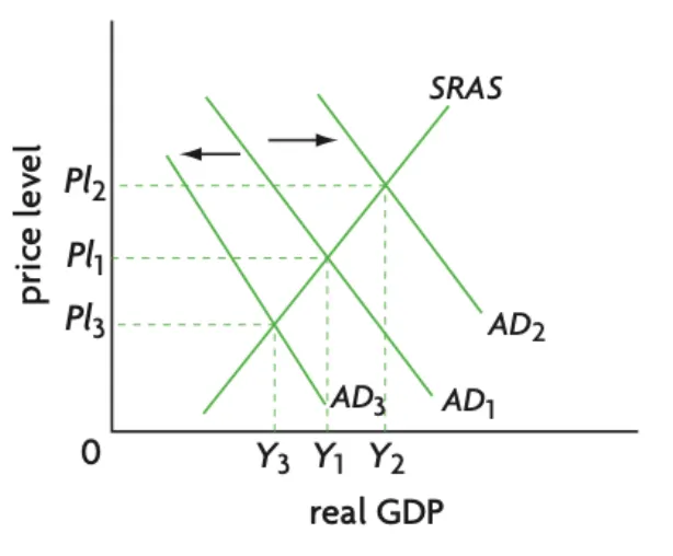
Shifts of the AD curve
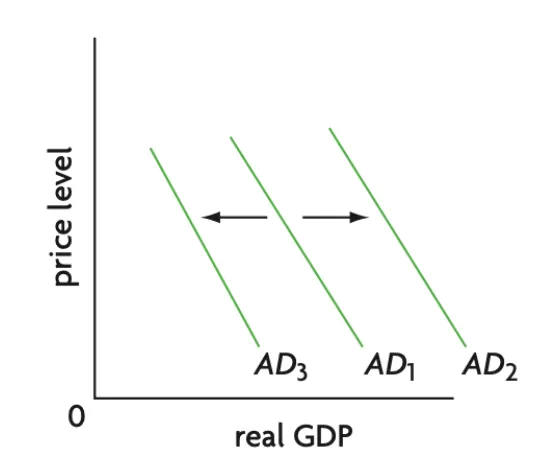
Figure 3.2.2 Shifts of the AD curve
•
AD will shift only if the determinant causes a change (increase or decrease) in the components of AD.
•
AD1 → AD2: increase in AD.
•
AD1 → AD3: decrease in AD.
Determinants of AD components
•
Consumption expenditures (C): spending by households on durables and nondurables and services
◦
Interest rates:
▪
Interest rate ↑ → cost of borrowing → C ↓
◦
Consumer confidence:
▪
▪
Confidence ↑ → C ↑
◦
Household wealth:
▪
Wealth ↑ → C ↑
◦
Personal income tax:
▪
Income tax ↑ → disposable income ↑ → C ↓
◦
Household indebtedness:
▪
Indebtedness ↑ → C ↓
◦
Expectations of future price level:
▪
Households expect future price levels ↑ → C ↑
•
Investment expenditures (I): spending by firms on capital goods per period of time.
◦
Interest rates:
▪
Interest rates ↑ → borrowing cost to finance the purchase of capital goods ↑ → I ↓
◦
Business confidence
▪
Confidence ↑ → I ↑
◦
Technology
▪
Fast improvement in technology → I ↑
◦
Business tax
▪
Business tax ↓ → profitability of business projects ↑ → I ↑ .
◦
Corporate indebtedness
▪
Indebtedness ↑ → I ↓
•
Government expenditure (G):
◦
Current spending on goods and services.
◦
Capital spending.
◦
Transfer payments: pension, unemployment benefits.
•
Net exports (X-M): Difference between spending by foreigners on domestic output minus domestic spending on foreign output or difference between export revenues and import expenditures per period of time.
◦
Income of trading partners
incomes of trading partners ↑ → spending on exports ↑ → X-M ↑ →
Exchange rates
•
Trade policies: restrictions to international trade (e.g. tariffs, quotas).
Imposition of tarrif or quota → imports → X-M ↑
Aggregate supply
Aggregate supply(AS): total level of output domestic firms are willing to offer at average price levels per period of time.
AS under the monetarist/new classical model
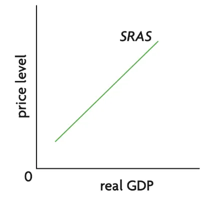
Short-run aggregate supply
Short-run(SR): the period during which money wages are fixed and unable to adjust to changes in the price level.
The shape of the SRAS curve is upward sloping
•
If the average price level (APL) increases, real wage decreases (i.e. wage adjusted to levels of inflation drops), so firms are able to offer more output.
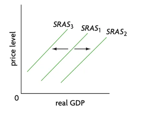
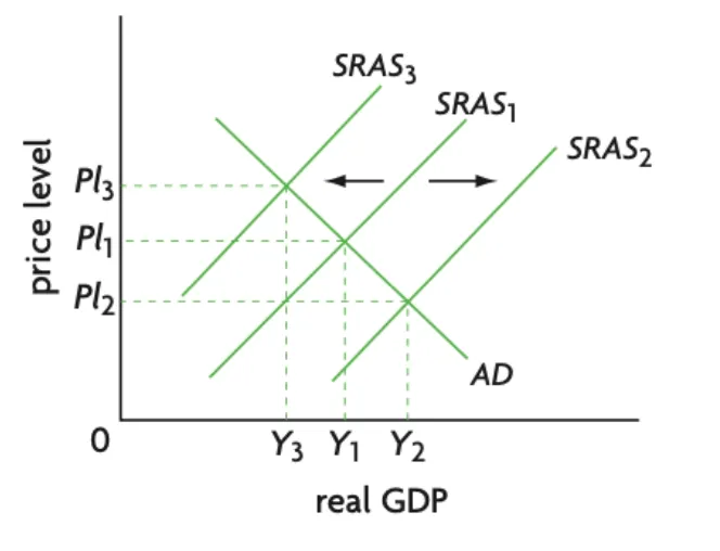
SRAS curve shifts due to:
•
Money wages change - i.e. change in the minimum wage: money wage ↑ → firm’s production cost ↓ → SRAS ↓ → leftward shift of SRAS curve (SRAS1 → SRAS3).
•
Energy price change: oil price change: oil price ↑ → firm’s production cost ↓ → SRAS ↓ → leftward shift of SRAS curve (SRAS1 → SRAS3).
Indirect tax or subsidy change: indirect tax ↑ → cost of production ↑ → SRAS ↓ → leftward shift of SRAS curve (SRAS1 → SRAS3).
Long-run aggregate supply
Long-run(LR): money wages are assumed to be flexible and able to fully adjust to changes in the price level.
The shape of the LRAS curve is vertical
•
Changes in APL don’t affect real output because real wage is not affected (i.e. wage can fully adjust to changes in the price level).
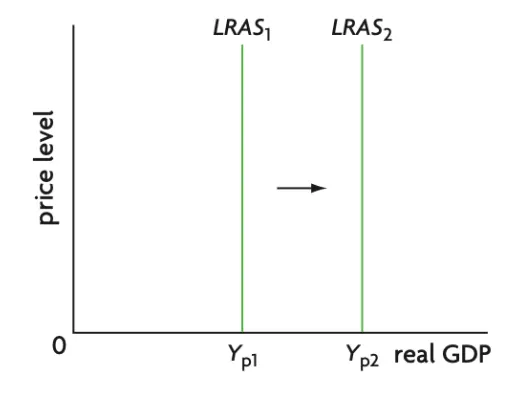
LRAS curve shifts due to:
•
Change in quality of factors of production: greater education level → quality of labour ↑ → LRAS ↑ → rightward shift of LRAS curve (LRAS → LRAS’).
•
Change in quantity of factors of production: immigration → quantity of labour ↑ → LRAS ↑ → rightward shift of LRAS curve (LRAS → LRAS’).
•
Improvement in technology: technological innovation → improved machines and equipment → able to produce more output → rightward shift of LRAS curve (LRAS → LRAS’).
•
Efficiency ↑ → produces a greater quantity of output → rightward shift of LRAS curve (LRAS → LRAS’).
•
Institutional change - improvements in institutional framework → economy’s productive capacity ↑ → rightward shift of LRAS curve (LRAS → LRAS’).
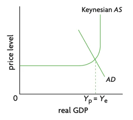
Aggregate supply under the Keynesian model
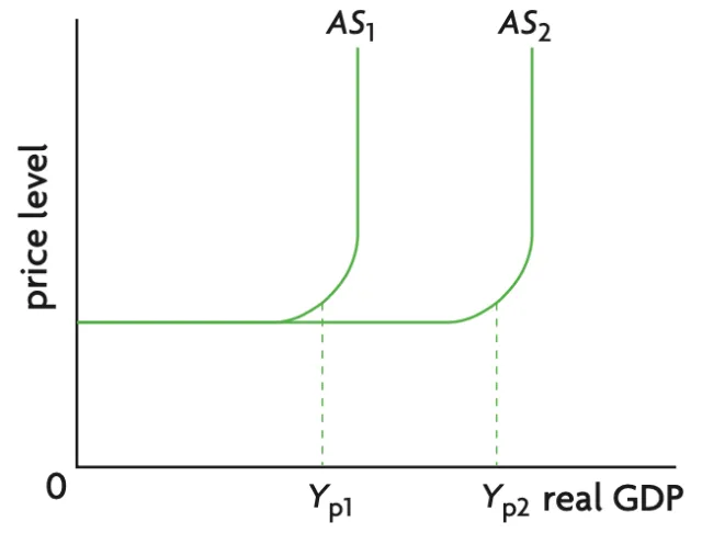
Figure 3.2.3 Aggregate supply curve (Keynesian)
•
Section I: horizontal - higher levels of output are produced without the average price level (APL) rising.
•
Section II: upward sloping AS curve - some economies may reach full employment faster than others.
•
Section III: vertical at the full employment level of output (Yf) - no unemployment in the economy.
◦
Real output cannot increase beyond Yf.
Macroeconomic equilibrium
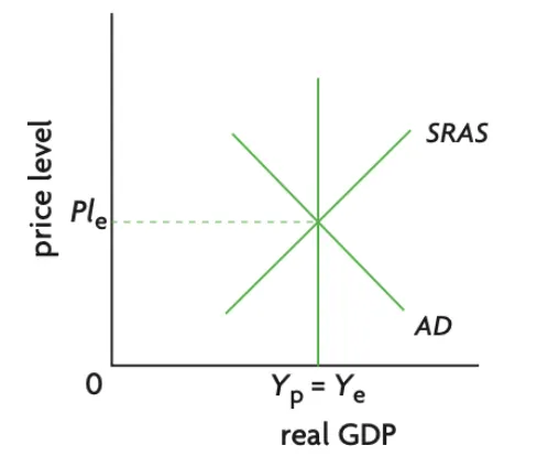
Equilibrium in the Monetarist / New Classical model
Short-run equilibrium
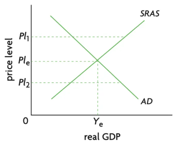
Exists at the level of output at which AD is equal to SRAS.
A shift in AD → changes the equilibrium average price and output levels in the same direction as the shift in AD.
Shift in SRAS → changes the average price level and output levels in the opposite direction as the shift in SRAS.
Long-run equilibrium
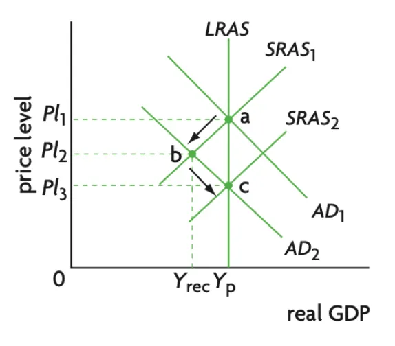
•
A: real output is at its potential level (Yp), unemployment is at its natural level (NRU), and the average price level is at APL.
•
A→B: business & consumer confidence decrease → consumption & investment expenditure decrease → AD decrease (AD1 → AD2) → average price level decrease (APL1 → APL2).
Deflationary gap (recessionary gap): exists when equilibrium real output is below the potential (full employment) level of output.
Inflationary gap:
exists when equilibrium real output is greater than potential (full employment) output.
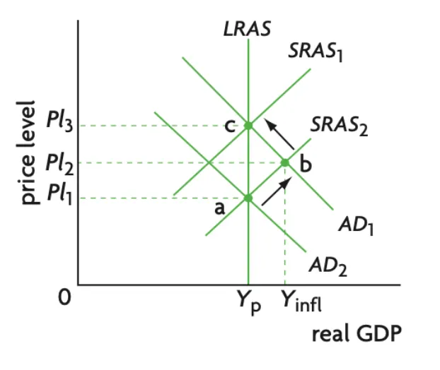
•
Money wages are assumed to be flexible in the long run → real wage returns to its original level → unemployment returns to its natural level (NRU) → economy automatically moves to A3.
Equilibrium in the Keynesian model
•
Money wages are assumed to be ‘sticky downwards’ - AD is the driving force behind the equilibrium level of economic activity.
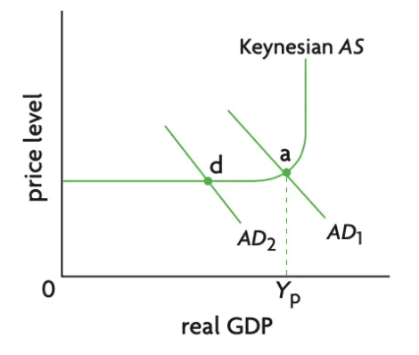
Deflationary gap: between Yr2 & Yf
•
Initial: full employment (Yf).
•
Money wages are ‘sticky downwards’ - i.e. the economy may remain stuck in a deflationary gap.
•
Government must intervene in order to restore full employment.
◦
Expansionary fiscal policy.
◦
Expansionary monetary policy.
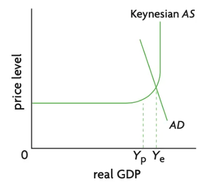
Inflationary gap: vertical distance between a & b
•
Initial: the economy is at full employment level of output Yf
•
Business & consumer confidence ↑ → rightward shift of AD (AD1 → AD2) → equilibrium real output remains at Yf // APL ↑ (APL1 → APL2).
Inflationary gap: between Yfe & Y1
•
Incorporates idea of the natural rate of unemployment.