

Gallery view
Search
How to measure economic activity
Gross Domestic Product (GDP)
: the value of all final goods and services produced within an economy over a period of time, usually a year or a quarter.
Output approach | Expenditure approach | Income approach |
adds up the value of all the final goods and services produced by each economic sector | adds up the total amount spent on domestically produced final goods and services | adds up all the income generated in the production process and by the factors of production in the economy |
GDP = sector 1 + sector 2 + sector 3 + … + sector n | GDP = C + I + G + (X-M)
• C = consumption spending
• I = investment spending
• G = government spending
• X-M = net export | GDP = rent + wage + interest + profit |
•
Gross National Income (GNI):
GDP+ factor income from abroad − factor income sent abroad.
•
GDP or GNI per capita: population of the country GDP or GNI
◦
Measures standard of living of a country.
•
Real GDP or GNI per capita at purchasing power parity (PPP): converts each country’s per capita income figure to a common currency.
Real vs Nominal:
Real GDP | Nominal GDP |
Nominal GDP adjusted for inflation | Measures economic activity in monetary terms, at current prices. |
GDP deflator: comprehensive price index that measures the average level of prices of all goods and services included in the GDP of a country.
GDP deflator = real GDP nominal GDP ×100
Real GDP = GDP deflator nominal GDP ×100
3.1. Measuring economic activity and illustrating its variations
Aggregate demand
Aggregate demand(AD): total spending on domestic goods and services at average price levels per period of time.
•
AD = C + I + G + (X-M)
◦
C = consumption expenditures
◦
I = investment expenditures
◦
G = government expenditures
◦
X-M = net export (export - import)
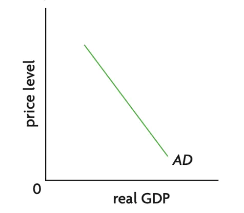
Figure 3.2.1 The aggregate demand curve
Why is the AD curve downward sloping?
Wealth effect | Trade effect | Interest rate effect |
average price level(APL) ↑ → real value of money people possess ↓ (i.e. people feel ‘poorer’) → consumer expenditure (C) ↓ → C is a component of AD → upward movement along AD | APL ↑ → exports become less competitive abroad // imports seem more attractive at home country → value of net export (X-M) ↓ → X-M is component of AD → upward movement along AD . | APL ↑ → demand for holding money ↑ → C and investment expenditure (I) ↓
(i.e. people and firms will borrow less from banks to buy durables and capital equipment) → C & I are components of AD → upward movement along AD . |
Shifts of the AD curve
3.2 Variations in economic activity: aggregate demand and aggregate supply
Economic growth
Economic growth: increase of real GDP over time.
Growth 22019→2020=rCDP19rGDP20−rGDP19×100
•
Growth rate = % change of real GDP between two periods.
Assume that real GDP in 2019 = $19,220 billion & real GDP in 2018 = $18,783 billion.
Growth in 2019=1878319220−18783×100=2.33%
Growth over the short term
•
AD increase → real GDP increase.
◦
Any factor that increases any component of AD will shift it to the right and increase real output.
◦
AD = C + I + G + (X-M).
A. Improved consumer & business confidence → C & I ↑ → C & I are components of AD → AD ↑ → real GDP ↑ → economic growth ↑ in short term.
B. Interest rates ↓→ ↓cost of borrowing for households and firms → C & I ↑ → C & I are components of AD → AD ↑→ real GDP ↑ → economic growth ↑ in short term.
1.
Interest rates ↓→ exchange rate depreciation → exports cheaper & more competitive // imports more expensive & less attractive → X-M ↑ → X-M is component of AD → AD ↑ → real GDP ↑ → economic growth ↑ in short term.
C. G ↑ → G is component of AD → AD ↑.
D. Tax ↓ → disposable income ↑ → C ↑.
E. Exchange rate depreciation → X-M ↑.
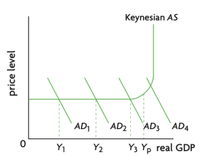
Figure 3.3.1 Short term growth on the Keynesian model
3.3 Macroeconomic objectives
Measuring economic inequality
Economic inequality:
unequal distribution of income and wealth.
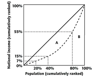
Figure 3.4.1 Lorenz curve
•
The poorest 20% of people receives only 7% of national income.
•
Diagonal line: line of perfect income equality (i.e. poorest 20% earns 20% of income and the poorest 40% earns 40% of income).
•
As we move further to the right of the diagonal, the distribution of income becomes more and more unequal.
Gini coefficient: ratio of the area between the Lorenz curve and the diagonal over the area of the half-square.
3.4 Economics of inequality and poverty
Functions of money
•
Medium of exchange
◦
Acceptable as a means of payment in all market transactions.
•
Unit of account
◦
Express prices → measure and compare values of goods and services.
•
Store of value
◦
Hold purchasing power and wealth over time.
•
Standard of deferred payment
3.5 Demand management (demand-side policies): monetary policy
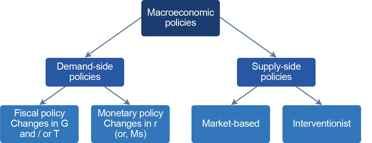
Fiscal policy: changes in the level of government expenditures (G) and taxes (T) to affect AD.
Government expenditures
Capital expenditures | Current expenditures | Transfer payments |
Public investments: spending on infrastructure (roads, airports). | Salaries of public sector employees Expenditures on public school, hospital. | Pensions, unemployment benefits. |
Government revenues
Where government gets its revenue from:
•
Direct tax.
•
Indirect tax.
•
Sale of state owned enterprises (by privatisation).
Goals of fiscal policy
•
Lift an economy from recession: close a large recessionary or inflationary gap.
•
Decrease cyclical unemployment.
◦
Lift an economy from recession → higher demand for employers → lower unemployment.
•
Decrease inflation.
•
Long-term economic growth.
3.6 Demand management (demand-side policies): fiscal policy Fiscal policy
Supply-side policies: attempt to shift LRAS to the right and achieve long-run economic growth.
Goals of supply-side policies
Goal | Explanation |
Increase the productive capacity. | Increase potential output by rightward shift of the LRAS curve. |
Improve competition and efficiency. | Make the economy more responsive to the forces of demand and supply so as to increase efficiency in production. |
Reduce labour costs and unemployment through labour market flexibility. | Make labour market more responsive to the forces of demand and supply so as to reduce unemployment as well as labour costs. |
Increase incentive of firms to invest in innovation. | Lower cost of production provide firms with incentives to engage in research and development (R&D) which increases the productive capacity of the economy. |
Reduce inflation to improve international competitiveness. | Reduce inflationary pressure in the economy, which makes exports more competitive in global markets. |
Market-based policies
Product market related policies
Anti-monopoly regulation | Deregulation | Privatisation | Trade liberalisation |
Establish competition commissions, pass antitrust laws. | Relax inappropriate rules, restrictions, and laws in the operation of firms / markets.
• Airline, banking, and electricity industries. | Transfer of state-owned assets to the private sector.
• Utilities: water, electricity.
• Privately owned firms pursue profit maximisation → operate more efficiently. | Elimination of policies that protect domestic firms from foreign competition.
• Tariff
• Quotas
• Subsidies
• Health & safety barriers |
Labour market related policies
Reduce power of labour unions | Decrease or abolish minimum wage | Reduce non-wage labour costs |
Decrease money wages and production costs.
• Firms reduce prices and increase output. | Decrease production costs → lower prices → increase output → increase investment. | Employer contributions to national insurance, pension schemes. |
Incentive-related policies
Cut personal income tax | Cut business tax and capital gains tax |
Increase labour supply: more individuals join the labour force → shift LRAS curve to the right. | Increase profitability of investments → increase potential output → shift LRAS curve to the right. |
Interventionist supply-side policies
Increase public investments in education, training, healthcare | Public investment in infrastructure | Public investment in research and development (R&D) |
Increase stock and quality of human capital: education, training, skills, experience | Infrastructure: physical capital that decreases the overall cost of economic activity.
• Better transportation network.
• Electrification → access to information. | Spillover benefits
• Invest R&D in the form of subsidies, tax allowances, and patents. |
Industrial policies
3.7 Supply-side policies
Economic growth
Fiscal policy
Strengths | Weaknesses |
Increase in government expenditures (G), decrease in taxes (T) → increase AD: expansionary fiscal policy → promote economic growth. | Long time lags
• Not effective during a recession. |
Monetary policy
Strengths | Weaknesses |
Decrease in interest rates → increase AD → increase real GDP: promote economic growth. | Limited ability to stimulate growth
• If interest rates are close to 0, then there’s limited scope to decrease interest rates. |
Flexible, incremental, reversible, short time lags: better than monetary policy as a short-run stabilisation tool. | Not effective during deep recession
• Very low consumer and business confidence. |
Supply-side policy
Strengths | Weaknesses |
Public investments in infrastructure, education, healthcare → accelerate economic growth. | Huge opportunity cost. |
Low and stable rate of inflation
Fiscal policy
Strengths | Weaknesses |
Contractionary fiscal policy:
Decrease G, increase T → AD ↓ → inflation ↓ | After excessive government expenditures: Tighter monetary policy → inflationary pressures. |
Monetary policy
Strengths | Weaknesses |
Increase interest rates → price stability. | Ineffective to deal with deflation
• Interest rates are already low (close to 0). |
Supply-side policy
Strengths | Weaknesses |
More flexible labour markets
• Increase productive capacity → reduce inflation. | Long time lags
• Further increase inflationary pressures Takes long time for policies to come into effect. |
3.8 Macroeconomic policies - strengths, limitations and conflicts