

Economic growth
Economic growth: increase of real GDP over time.
•
Growth rate = % change of real GDP between two periods.
Assume that real GDP in 2019 = $19,220 billion & real GDP in 2018 = $18,783 billion.
Growth over the short term
•
AD increase → real GDP increase.
◦
Any factor that increases any component of AD will shift it to the right and increase real output.
◦
AD = C + I + G + (X-M).
A. Improved consumer & business confidence → C & I ↑ → C & I are components of AD → AD ↑ → real GDP ↑ → economic growth ↑ in short term.
B. Interest rates ↓→ ↓cost of borrowing for households and firms → C & I ↑ → C & I are components of AD → AD ↑→ real GDP ↑ → economic growth ↑ in short term.
1.
Interest rates ↓→ exchange rate depreciation → exports cheaper & more competitive // imports more expensive & less attractive → X-M ↑ → X-M is component of AD → AD ↑ → real GDP ↑ → economic growth ↑ in short term.
C. G ↑ → G is component of AD → AD ↑.
D. Tax ↓ → disposable income ↑ → C ↑.
E. Exchange rate depreciation → X-M ↑.
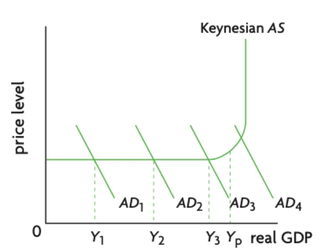
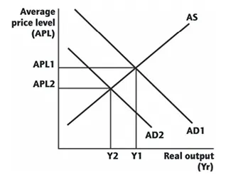
Figure 3.3.1 Short term growth on the Keynesian model
•
AD ↑ (AD1 → AD2) → average price level (APL) doesn’t increase.
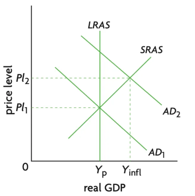
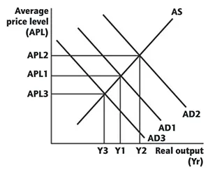
Figure 3.3.2 Short run growth in the monetarist/new classical model
•
Economy operates past potential real output → AD ↑ (AD1 → AD2) is not effective.
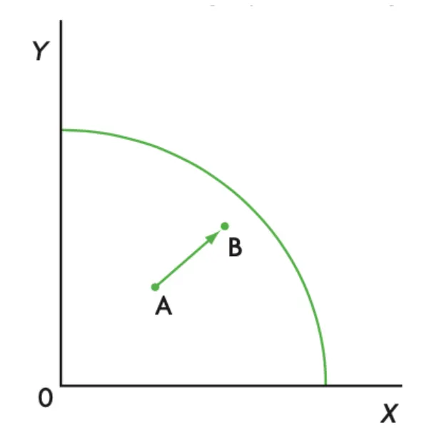
Figure 3.3.3 Economic growth as an increase in actual output caused by reductions in unemployment and productive inefficiency
•
A → B: Good X & Y being more produced.
◦
Greater total output.
•
The closer an economy is to its PPC, the lower the resource unemployment and productive inefficiency.
•
Reducing unemployment and increasing productive efficiency bring the economy closer to its PPC and increase the actual quantity of output produced.
•
Movement from a point like A to B in Figure 11.1(a) illustrates the growth of actual output.
Growth over the long term
•
Increase in population / influx of migrant workers / increase in the participation of some population group Labour force size increase.
•
Investment in education & healthcare → labour productivity increase.
•
More and better infrastructure becoming available → stock of physical capital increase → more machines and factories → economy’s productive capacity increase.
•
Technological advancements.
•
Information & communication technologies (ICT) advancements.
•
Institutional framework improvements - e.g. less bureaucracy, more flexible labour market, more competition in the labour markets.
Keynesian model
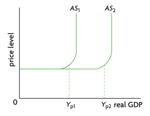
Rightward shift of the AS curve.
Monetarist/New Classical model
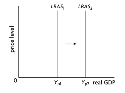
Rightward shift of the LRAS curve.
Production possibilities curve (PPC)
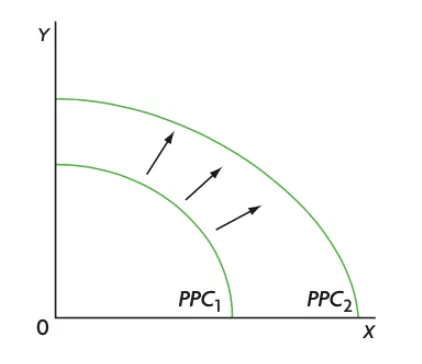
Outward shift of PPC - able to produce combinations of goods that initially were not feasible.
Consequences of economic growth
Impact of economic growth on living standards
•
Economic growth doesn’t imply improved living standards for the population - may only apply to the wealthiest
•
Economic growth negatively impacts the environment → economic growth doesn’t necessarily improve living standards
Impact of economic growth on the environment
•
Positive impact: richer countries have more resources to deal with environmental issues
•
Negative impact: increased pollution, environmental degradation
•
Solution: governments stop subsidising use of fossil fuels, enforce stricter environmental regulations
Impact of economic growth on the distribution of income
Decrease income inequality (positive impact) | Increase income inequality (negative impact) |
Economic growth → higher incomes → higher income & expenditure tax collected → higher tax revenue for government → governments adopt policies that alleviate poverty | Economic growth only driven by certain industries / regions of a country = ‘skill-biassed technological progress’ → wages of the highly skilled workers rise faster than wages of the less skilled |
Economic growth → governments can invest in programmes to lift people out of poverty → decrease income inequality | Economic growth → increase in corporate concentration and monopoly power- i.e. firms with high monopoly power charge consumers more for products & pay their workers less |
Economic growth → increased trade liberalisation and globalisation → workers in import-competing industries lose their income // workers in export-oriented industries increase their income |
Low unemployment
Difficulties of measuring unemployment
•
Some individuals conceal their true employment status.
•
Some individuals are employed in illegal activities → reported that they are unemployed.
•
Underemployed individuals - i.e. involuntary part-time workers.
•
Discouraged workers - individuals who have stopped actively searching for a job because their past job search effort has been unsuccessful.
Causes of unemployment
Seasonal unemployment: a result of unavoidable and predictable variations in the demand and supply of labour.
•
Construction workers being seasonally unemployed in winter months: freezing temperatures and ice may prevent their work → increasing the risk of work-related accidents.
Frictional unemployment: people who are between jobs as it takes time to match a job-seeker with an available job vacancy.
•
Short-term, unavoidable.
•
Solution: ensure that job vacancies as well as the profiles of those available for work become known wider and faster (e.g. via the internet).
Cyclical (demand deficient) unemployment
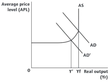
Figure 3.3.4 Cyclical unemployment
•
Initial: the economy is assumed to be at Yf (full employment level of output).
•
AD decrease (AD → AD’) → real output decreases below full employment (Yf → Y’) → def lationary gap forms (Y’Yf) → cyclical unemployment .
Structural unemployment: caused by a change in the structure of the economy which causes a mismatch between the skills of those out of work and the skills needed to fill the available vacant jobs.
•
Long term problem.
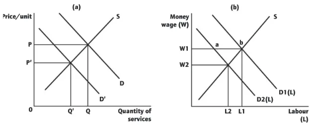
Figure 3.3.5 Structural unemployment
•
Figure (a): demand for a particular industry ↓ (D → D’) → less quantity produced (Q → Q’) & lower price (P → P’).
•
Figure (b): demand for labour ↓ (D1(L) → D2(L)) → if money wages are “sticky downwards” (wages remain at W1) then structural unemployment (ab).
◦
Money wages ↓ (W1 → W2) → less labour demanded (L1 → L2).
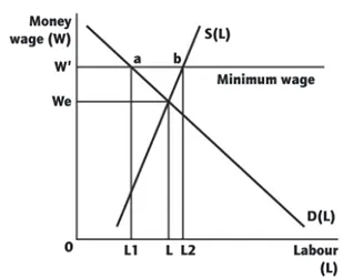
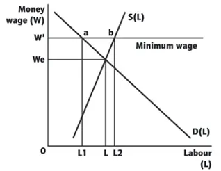
Figure 3.3.6 Structural unemployment due to minimum wage
•
Higher minimum wage (We → W’) → excess supply of labour (L2-L1 = ab) = structural unemployment.
Other labour market rigidities:
•
High unemployment benefits: disincentive unemployed to accept a job offer.
•
Laws that guarantee job security: more costly for firms to fire workers.
The natural rate of unemployment:
Occurs when labour market is at full employment, but there is still some residual frictional, seasonal and structural unemployment.
•
Economy is at the full employment level of output.
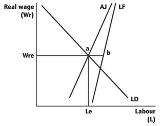
Figure 3.3.7 Natural rate of unemployment (b - a)
Costs of unemployment
Economic costs | Personal costs | Social costs |
Rising unemployment → tax revenue ↓ (due to income tax ↓) → unemployment benefit ↑ → government expenditure ↑ | Unemployment → lost income → unemployed people may lose their house → homeless. | Unemployment → crime & violence ↑ → negative externalities resulting from increased drug & alcohol abuse. |
High, prolonged unemployment → unemployed lose their income while others maintain their income → income inequality ↑ | Unemployment = losing job → losing health insurance. | |
High, prolonged unemployment → younger and better educated people ↓ → human capital ↓ → labour productivity ↓ | Unemployment → lose their skills → their job prospect ↓ → compete against others with up to date skills. | |
Long-term unemployment → family breakdown, alcohol abuse, loss of self esteem, suicide. |
Inflation
•
Inflation: sustained increase in the average price level.
•
Inflation rate: % change in the average price level between 2 periods.
•
Disinflation: decrease in the rate of inflation (slowdown in the rate of increase of the general price level of goods and services).
•
Deflation: sustained % fall in the general price level (fall in prices).
Measuring inflation
Consumer price index (CPI):
weighted index of the prices of a basket of goods and services consumed by typical households.
•
Inflation is measured by calculating CPI:
where the w’s are the weights and
Limitations of the CPI in measuring inflation
•
Index measuring inflation may not reflect the situation felt by an income group.
◦
Different groups of people buy different baskets of goods and services.
•
Improvements in quality are not taken into account by indexes.
•
Doesn’t take into account changes in consumption patterns.
•
New products that consumers buy are included in the CPI only after a significant time lag.
Consequences of a high inflation rate
Costs | Benefits |
Inflation increases the uncertainty that businesses face.
• It makes it difficult for firms to make judgments (e.g. whether an investment project will be profitable?). | Reduces the real value of debt.
• Households, firms, and government owe less in real terms. |
The real income of fixed income earners decreases.
• Individuals who can adjust their earnings might receive raised incomes → widens income inequality. | |
Reduces export competitiveness
• Exports become more expensive → less competitive in foreign markets.
• Imports become cheaper → more attractive to domestic buyers → import expenditure ↑.
• Lower export revenue (X) and increased import expenditure (M) → X-M ↓ → X-M is a component of AD → AD ↓ → trade deficit ↑ |
Causes of inflation
Definition
Cause
Diagram
Demand-pull inflation
AD increases faster than AS causing more demand for goods.
Proliferate government spending.
• government expenditure (G) ↑ → G is a component of AD → AD ↑ = demand-pull inflation.
Overly optimistic households and firms.
• Excessive consumer spending (C), investment spending (I) → C and I are components of AD → AD ↑ = demand-pull inflation.
Cost-push inflation
Increase in companies’ costs (labour and raw materials) which are passed onto the consumer in the form of higher prices
Decrease AS.
Increase in the price of oil.
• oil price ↑ → production cost for many firms ↑ → AS ↓ = cost-push inflation.
Powerful labour unions.
• money wages ↑ → production costs for firms ↑.
Deflation
Deflation: sustained decrease in the average price level = fall in prices.
Causes of deflation
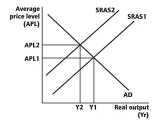
Sustained decrease in aggregate demand
AD ↓ (AD1 → AD2) → real output ↓ → (Y1 → Y2) → average price level ↓ (APL1 → APL2).
Increase in aggregate supply
AS ↑ → real output ↑ → average price level ↓ = ‘good deflation’.
Costs of deflation
Induce consumers to delay purchases of durables.
• Consumers expect further price falls. | Decrease firms’ revenues.
• Reduce profit margins → force firms to cut the cost of production → wages decrease. | Households and firms become hesitant to spend
• What households and firms owe to banks increases in real terms → consumer spending (C) & investment (I) ↓ → C & I are components of AD → AD ↓. | the Economy may enter a deflationary spiral
• Deflation creates more deflation. |
Government (national) debt
•
Budget deficit: government spending > taxation.
•
Budget surplus: taxation > government spending.
Costs of a high national debt
Cost of debt servicing | Credit ratings |
Debt servicing: paying back the principal & interest
• Carries a high opportunity cost.
• Service debt by issuing new money → increase risk of inflation → currency depreciation. | Credit ratings: grade assigned by certain agencies (e.g. Moody’s) on the borrowing risks a prospective debt issuer presents to lenders.
• Higher debt to GDP ratio → greater risk that a credit agency will downgrade the country’s bonds. |
The Phillips curve
Phillips curve: shows the trade-off between unemployment and inflation.
Economy is at equilibrium with Y1 + APL 1 → AD increase to AD2 → equilibrium real output increase to Y2.
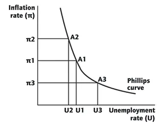
Some unemployment (U1) → AD ↑ (AD1 → AD2) → higher level of economic activity decrease unemployment (U1 → U2) → inflation ↑ (π1 → π2).
Long-run Phillips curve
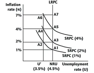
Figure 3.3.8 Long-run Phillips curve
•
Economy is initially at A1.
•
Government tries to decrease unemployment below the NRU by increasing AD.
•
Long run: money wages are assumed flexible → money wages ↑ → move to A5 with unemployment at NRU.