5.3 Application of Differential Calculus

Tags

Differentiation

Tangent

Optimization

Related rates

Kinematics

Euler's method

Maclaurin series

Trigonometric functions

Exponential and Logarithmic functions

Modelling

Graphs

Chain rule

Quotient rule

Product rule

There are different applications you need to be aware of.

Application

Steps

Tangents

Tangent at

a

denotes the best approximating straight line to the curve at

a

We must have two pieces of information to obtain the equation of a tangent:

Point of contact (a,f(a))(a, f(a))(a,f(a))

The gradient of a tangent at that point: f′(a) f'(a)f′(a)

Then, use

y - y_0 = m(x-x_0)

to obtain the equation of the tangent.

Rate of change

\frac {dy}{dx}

represents the rate of change in

y

respect to

x

Optimization

Represent the situation in a clear diagram. Label the variable.

Construct a formula with the variable to be optimized as a subject. Write down what domain restrictions there are on xxx.

Calculate the minimum or maximum depending on the situation.

Related rates (HL)

Represent the situation in a clear diagram. Label the variable. Identify which information you have, and what you need to calculate.

Construct a formula with the variable and obtain the derivative.

Substitute the values for the particular case.

*Note: angles must be in radian.

Kinematics is the study of motion; modeling and analyzing the motion of objects in a straight line.

Terms	Definition
Displacement $s$ m	A particle’s distance relative to a fixed point– usually the origin $s(t)$ Displacement is zero when the object is at or has returned to the origin Displacement can be positive or negative Displacement can be found by integrating velocity: $s(t)=v(t)dt$ Use given initial conditions to solve the constant $c$
Distance $d$ m	Distance is always positive Distance traveled from $a$ to $b$ can be found by: $\int_a^b\|v(t)\|dt$
Velocity $v$ ms⎺¹	The rate of change of a particle’s displacement at time $t$ $v(t)=\frac{ds}{dt}$ Velocity can be positive or negative depending on the direction of motion When the particle is stationary/ at rest, its velocity equals to zero Velocity can be found by differentiating $s(t)$ or integrating $a(t)$ $v(t)=\int a(t)dt$ Use given initial conditions to solve the constant $c$
Speed $\|v\|$ ms⎺¹	The magnitude or absolute value of velocity–thus neglecting the direction of a particle
Acceleration $a$ ms⎺²	The rate of change of a particle’s velocity at time $t$ $a(t)=\frac{dv}{dt}=\frac {d^2s}{dt^2}$

Euler’s Method (HL)

This is a numerical method to solve

\frac{dy}{dx}=f(x, y)

with particular solution

(x_0, y_0)

Given the initial value, choosing the step size

h

, we obtain the

i

th point:

xi=xi−1+hx_i=x_{i-1}+hxi​=xi−1​+h

yi=yi−1+hf(xi−1,yi−1)y_i=y_{i-1}+hf(x_{i-1}, y_{i-1})yi​=yi−1​+hf(xi−1​,yi−1​)

Figure 5.3.1 Numerical approximation of the gradients by Euler’s method

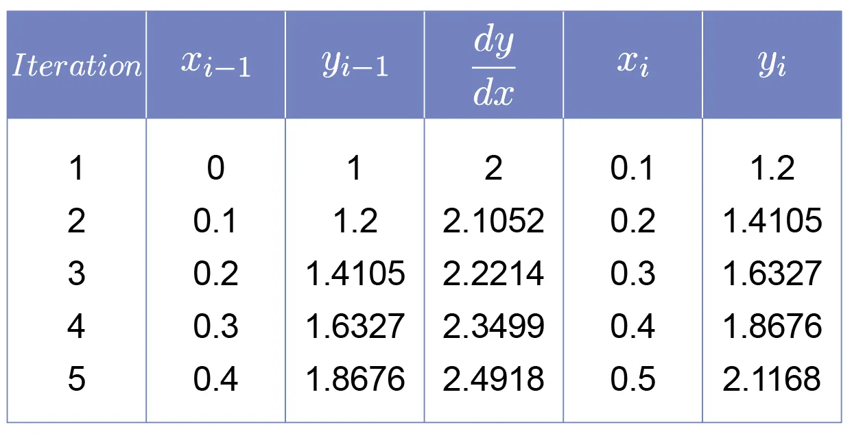
This creates a polygonal approximation to the solution curve.

We apply this iterative step n times to reach

x =b

n \rightarrow ∞

, from the fundamental theorem of calculus, we have:

y(b) =y(x_0)+\int_{x_0}^{b}\frac {dy}{dx}dx

Construct an appropriate table of each iteration to apply Euler’s method using the calculator.

The last application is a series expansion of function

f

, expressing

f

as an infinite sum of polynomials.

Maclaurin series (HL)

The Maclaurin series is a Taylor series expansion of a function about 0.

f(x)=\sum_{n=0}^∞\frac{f^{(n)}(0)x^n}{n!}=f(0)+f'(0)x+\frac{f^{(2)}(0)}{2!}x^2+\frac{ f^{(3)}(0)}{3!}x^3+ ...

There are different types of method to approach this:

Method	Steps
Definition	1. Differentiate $f$ multiple times to find the pattern. 2. Apply the result to the general form.
Composite function	1. Notice if you are given the form $f(g(x))$ 2. Substitute the Maclaurin series of $g$ into the Maclaurin series of $f$ , and simplify.
Integration	1. Notice that your function $f(x)$ can be found as an integration of a function of lower order, for instance, $g(x)$ . 2. Find the series of $g(x)$ and integrate to find $f$ . This is because the Maclaurin series is analytic, i.e. infinitely differentiable/integrable.

5.4 Applications of differential calculus

done

https://forms.gle/5tnTujiRR4nWvRcr9

5.3 Application of Differential Calculus