

Linear
General form:
Standard form:
From the standard form, we have:
1.
Slope, or Gradient: , the rate of change in relative to .
a.
: ascending rightwards
b.
: descending rightwards
c.
: horizontal line
2.
intercept:
3.
If and, then:
a.
b.
Quickest way to draw this function:
1.
Plot and intercepts.
2.
Connect the two intercepts.
Find intersection by solving the simultaneous equation. If and , solve:

The formula to find a linear function given a point ( ) and slope is:
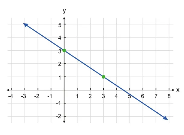
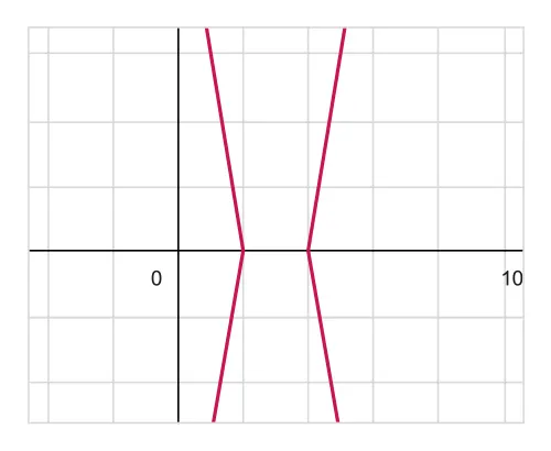
Figure 2.4.1 Graphical representation of a linear equation
Quadratics
General form:
Vertex form:
Intercept form:
From the standard form, we have:
1.
Axis of symmetry:
2.
Vertex: ()
3.
-intercept:
4.
For the sign of ,
a.
then concave up
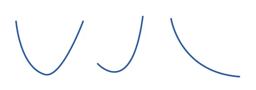
b.
then concave down

5.
Vertex marks the minimum/maximum of the graph depending on the concavity.
Quickest way to draw this function:
1.
Convert any other form to the vertex form:
2.
Plot the vertex ()
3.
Find the -intercept.
4.
Connect the vertex and -intercept with consideration of concavity.
To solve for the quadratic equation:
1.
Use to complete the square.
2.
Factorize where possible.
3.
Apply the quadratic formula.
Discriminant has three cases:
1.
: two real conjugate roots
2.
: repeated roots
3.
: two imaginary conjugate roots
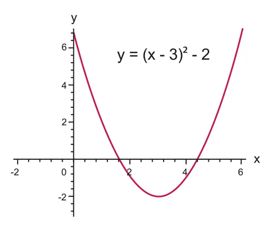
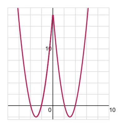
Figure 2.4.2 Quadratic function with two distinct real roots
Polynomials of degree (HL)
General form:
Degree: the highest power of the polynomial
We have several theorems for general polynomials:
Theorem | Features |
Euclidean Algorithm | We have and such that .
Notice that or |
Remainder theorem | If we divide by , then is the remainder. |
Factor theorem | If divides , then |
Fundamental theorem of Algebra | Over the field ℂ, the polynomial of degree has roots in ℂ.
The complex roots appear as conjugates, i.e. .
It follows that odd degree polynomial has at least one real root. |
Vieta’s theorem | Let the roots of be . Then, we have:
1. Sum of all roots:
2. Product of all roots: |
Modulus functions

denotes the absolute value of , the distance from 0 in the number line.
Some important properties are listed below:
1.
2.
3.
4.
or
5.
*Triangle inequality
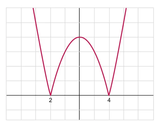
These are different forms of modulus function:
Features
Function
Reflect the region by the axis.
Reflect the region by the axis.
Reflect the region by the axis.
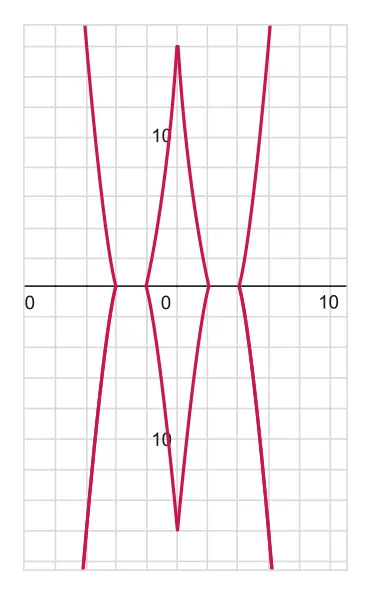
Draw the graph in the 1st quadrant, and reflect on all remaining quadrants.